1. Basics

The tensor network functionality in quimb aims to be versatile and interactive, whilst not compromising ease and efficiency. Some key features are the following:

• a core tensor network object orientated around handling arbitrary graph geometries including hyper edges

• a flexible tensor tagging system to structure and organise these

• dispatching of array operations to autoray so that many backends can be used

• automated contraction of many tensors using cotengra

• automated drawing of arbitrary tensor networks

Roughly speaking quimb works on five levels, each useful for different tasks:

1. ‘array’ objects: the underlying CPU, GPU or abstract data that quimb manipulates using autoray;

2. Tensor objects: these wrap the array, labelling the dimensions as indices and also carrying an arbitrary number of tags identifying them, such as their position in a lattice etc.;

3. TensorNetwork objects: these store a collection of tensors, tracking all index and tag locations and allowing methods based on the network structure;

4. Specialized tensor networks, such as MatrixProductState, that promise a particular structure, enabling specialized methods;

5. High level interfaces and algorithms, such as Circuit and DMRG2, which handle manipulating one or more tensor networks for you.

A more detailed breakdown of this design can be found on the page Design. This page introduces the basic ideas of the first three levels.

%config InlineBackend.figure_formats = ['svg']
import quimb as qu
import quimb.tensor as qtn

1.1. Creating Tensors

To create a Tensor you just need:

• data - a raw array, and

• inds - a set of ‘indices’ to label each dimension with.

Whilst naming the dimensions is useful so you don’t have to remember which axis is which, the crucial point is that tensors simply sharing the same index name automatically form a ‘bond’ or implicit contraction when put together. Tensors can also carry an arbitrary number of identifiers - tags - which you can use to refer to single or groups of tensors once they are embedded in networks.

For example, let’s create the singlet state in tensor form, i.e., an index for each qubit:

data = qu.bell_state('psi-').reshape(2, 2)
inds = ('k0', 'k1')
tags = ('KET',)

ket = qtn.Tensor(data=data, inds=inds, tags=tags)
ket

Tensor(shape=(2, 2), inds=[k0, k1], tags={KET}),

backend=numpy, dtype=complex128, data=array([[ 0. +0.j, 0.70710678+0.j], [-0.70710678+0.j, 0. +0.j]])

ket.draw()

This is pretty much like a n-dimensional array, but with a few key differences:

1. Methods manipulating dimensions use the names of indices, thus provided these are labelled correctly, their specific permutation doesn’t matter.

2. The underlying data object can be anything that autoray supports - for example a symbolic or GPU array. These are passed around by reference and assumed to be immutable.

Some common Tensor methods are:

• Tensor.reindex

• Tensor.retag

• Tensor.fuse

• Tensor.squeeze

• Tensor.gate

• Tensor.isel

• Tensor.new_ind

• Tensor.transpose

• Tensor.trace

• Tensor.norm

Hint

Many of these have inplace versions with an underscore appended, so that ket.transpose_('k1', 'k0') would perform a tranposition on ket directly, rather than making a new tensor. The same convention is used for many TensorNetwork methods.

Let’s also create some tensor paulis, with indices that act on the bell state and map the physical indices into two new ones:

X = qtn.Tensor(qu.pauli('X'), inds=('k0', 'b0'), tags=['PAULI', 'X', '0'])
Y = qtn.Tensor(qu.pauli('Y'), inds=('k1', 'b1'), tags=['PAULI', 'Y', '1'])

And finally, a random ‘bra’ to complete the inner product:

bra = qtn.Tensor(qu.rand_ket(4).reshape(2, 2), inds=('b0', 'b1'), tags=['BRA'])

Note how repeating an index name is all that is required to define a contraction. If you want to join two tensors and have the index generated automatically you can use the function qtn.connect.

Note

Indices and tags should be strings - though this is currently not enforced. A useful convention is to keep inds lower case, and tags upper. Whilst the order of tags doesn’t specifically matter, it is kept internally as a ordered set - oset - so that all operations are deterministic.

1.2. Creating Tensor Networks

We can now combine these into a TensorNetwork using the & operator overload:

TN = ket.H & X & Y & bra
print(TN)

TensorNetwork([
    Tensor(shape=(2, 2), inds=('k0', 'k1'), tags=oset(['KET'])),
    Tensor(shape=(2, 2), inds=('k0', 'b0'), tags=oset(['PAULI', 'X', '0'])),
    Tensor(shape=(2, 2), inds=('k1', 'b1'), tags=oset(['PAULI', 'Y', '1'])),
    Tensor(shape=(2, 2), inds=('b0', 'b1'), tags=oset(['BRA'])),
], tensors=4, indices=4)

(note that .H conjugates the data but leaves the indices). We could also use the TensorNetwork constructor, which takes any sequence of tensors and/or tensor networks, and has various advanced options.

The geometry of this network is completely defined by the repeated indices forming edges between tensors, as well as arbitrary tags identifying the tensors. The internal data of the tensor network allows efficient access to any tensors based on their tags or inds.

Warning

In order to naturally maintain networks geometry, bonds (repeated indices) can be mangled when two tensor networks are combined. As a result of this, only exterior indices are guaranteed to keep their absolute value - since these define the overall object. The qtn.bonds function can be used to find the names of indices connecting tensors if explicitly required.

Some common TensorNetwork methods are:

• TensorNetwork.reindex

• TensorNetwork.retag

• TensorNetwork.gate_inds

• TensorNetwork.isel

• TensorNetwork.trace

• TensorNetwork.contract

• TensorNetwork.norm

Note that many of these are shared with Tensor, meaning it is possible to write many agnostic functions that operate on either.

Any network can also be drawn using TensorNetwork.draw, which will pick a layout and also represent bond size as edge thickness, and optionally color the nodes based on tags.

TN.draw(color=['KET', 'PAULI', 'BRA', 'X', 'Y'], figsize=(4, 4), show_inds='all')

Note the tags can be used to identify both paulis at once. But they could also be uniquely identified using their 'X' and 'Y' tags respectively:

A detailed guide to drawing can be found on the page Drawing.

1.3. Graph Orientated Tensor Network Creation

Another way to create tensor networks is define the tensors (nodes) first and the make indices (edges) afterwards. This is mostly enabled by the functions Tensor.new_ind and Tensor.new_bond. Take for example making a small periodic matrix product state with bond dimension 7:

L = 10

# create the nodes, by default just the scalar 1.0
tensors = [qtn.Tensor() for _ in range(L)]

for i in range(L):
    # add the physical indices, each of size 2
    tensors[i].new_ind(f'k{i}', size=2)

    # add bonds between neighbouring tensors, of size 7
    tensors[i].new_bond(tensors[(i + 1) % L], size=7)

mps = qtn.TensorNetwork(tensors)
mps.draw()

Hint

You can also add tensors or tensor networks in-place to an existing tensor using the following syntax:

# add a copy of ``t``
tn &= t

# add ``t`` virtually
tn |= t

1.4. Contraction

Actually performing the implicit sum-of-products that a tensor network represents involves contraction. Specifically, to turn a tensor network of \(N\) tensors into a single tensor with the same ‘outer’ shape and indices requires a sequence of \(N - 1\) pairwise contractions. The cost of doing these intermediate contractions can be very sensitive to the exact sequence, or ‘path’, chosen. quimb automates both the path finding stage and the actual contraction stage, but there is a non-trivial tradeoff between how long one spends finding the path, and how long the actual contraction takes.

Warning

By default, quimb employs a basic greedy path optimizer that has very little overhead, but won’t nearly be optimal on large or complex graphs. See Contraction for more details.

To fully contract a network we can use the ^ operator, and the ... object:

TN ^ ...

(0.06766823867678032-0.8460798111575898j)

Or if you only want to contract tensors with a specific set of tags, such as the two pauli operators, supply a tag or sequence of tags:

TNc = TN ^ 'PAULI'
TNc.draw('PAULI')
print(TNc)

TensorNetwork([
    Tensor(shape=(2, 2), inds=('k0', 'k1'), tags=oset(['KET'])),
    Tensor(shape=(2, 2), inds=('b0', 'b1'), tags=oset(['BRA'])),
    Tensor(shape=(2, 2, 2, 2), inds=('k0', 'b0', 'k1', 'b1'), tags=oset(['PAULI', 'X', '0', 'Y', '1'])),
], tensors=3, indices=4)

Note how the tags of the Paulis have been merged on the new tensor.

The are many other contraction related options detailed in Contraction, but the core function that all of these are routed through is tensor_contract. If you need to pass contraction options, such as the path finding strategy kwarg optimize, you’ll need to call the method like tn.contract(..., optimize='auto-hq').

One useful shorthand is the ‘matmul’ operator, @, which directly contracts two tensors:

ta = qtn.rand_tensor([2, 3], inds=['a', 'x'], tags='A')
tb = qtn.rand_tensor([4, 3], inds=['b', 'x'], tags='B')

# matrix multiplication but with indices aligned automatically
ta @ tb

Tensor(shape=(2, 4), inds=[a, b], tags={A, B}),

backend=numpy, dtype=float64, data=array([[-1.82145456, 5.37156602, -0.6407701 , 1.73704458], [-3.04900789, 5.68378085, -3.08717877, 4.09540662]])

Since the conjugate of a tensor network keeps the same outer indices, this means that tn.H @ tn is always the frobenius norm squared (\(\mathrm{Tr} A^{\dagger}A\)) of any tensor network.

# get a normalized tensor network
psi = qtn.MPS_rand_state(10, 7)

# compute its norm squared
psi.H @ psi  # == (tn.H & tn) ^ ...

1.0

1.5. Decomposition

A key part of many tensor network algorithms are various linear algebra decompositions of tensors viewed as operators mapping one set of ‘left’ indices to the remaining ‘right’ indices. This functionality is handled by the core function tensor_split.

# create a tensor with 5 legs
t = qtn.rand_tensor([2, 3, 4, 5, 6], inds=['a', 'b', 'c', 'd', 'e'])
t.draw(figsize=(3, 3))

# split the tensor, by grouping some indices as 'left'
tn = t.split(['a', 'c', 'd'])
tn.draw(figsize=(3, 3))

There are many options that can be passed to tensor_split() such as:

• which decomposition to use

• how or whether to absorb any singular values

• specific tags or inds to introduce

Often it is convenient to perform a decomposition within a tensor network, here we decompose a central tensor of an MPS, introducing a new tensor that will sit on the bond:

psi = qtn.MPS_rand_state(6, 10)
psi.draw()

psi.split_tensor(
    # identify the tensor
    tags='I2',
    # here we give the right indices
    left_inds=None,
    right_inds=[psi.bond(2, 3)],
    # a new tag for the right factor
    rtags='NEW',
)

psi.draw('NEW')

1.5.1. Gauging

A key aspect of tensor networks is the freedom to ‘gauge’ bonds - locally change tensors whilst keeping the overall tensor network object invariant. For example, contracting \(G^{-1}\) and \(G\) into adjacent tensors (you can do this explicitly with TensorNetwork.insert_gauge).

A common example is ‘isometrizing’ a tensor with respect to all but one of its indices and absorbing an appropriate factor into its neighbor to take this transformation into account. A common way to do this is via the QR decomposition:

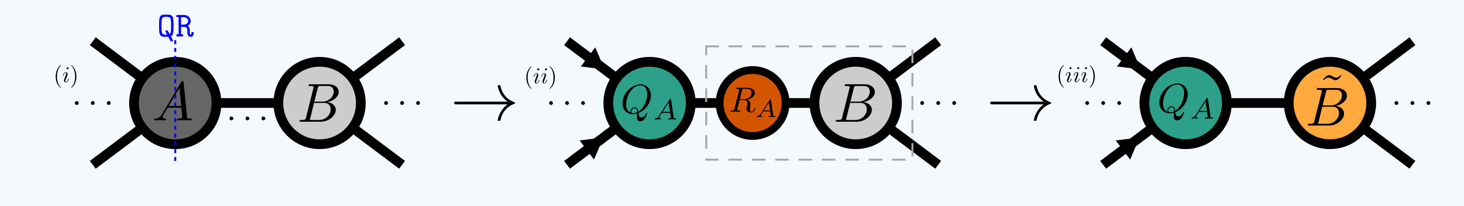
where the inward arrows imply:

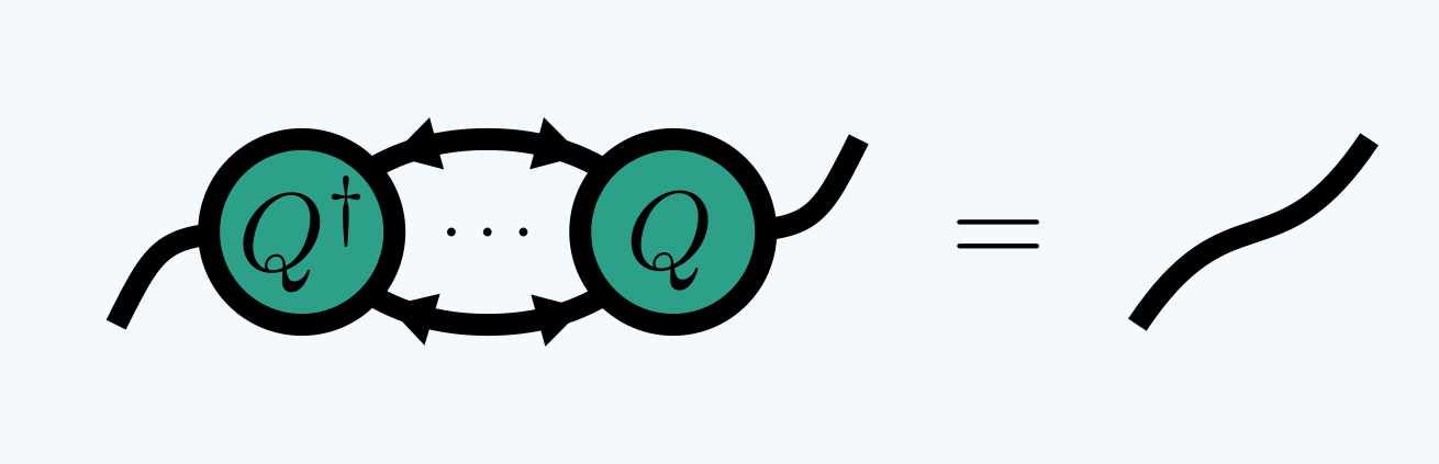
In quimb this is called ‘canonizing’ for short. When used in an MPS for example, it can used to put the TN into a canonical form, but this is generally not possible for ‘loopy’ TNs. The core function that performs this is qtn.tensor_canonize_bond.

ta = qtn.rand_tensor([4, 4, 4], ['a', 'b', 'c'], 'A')
tb = qtn.rand_tensor([4, 4, 4, 4], ['c', 'd', 'e', 'f'], 'B')

qtn.tensor_canonize_bond(ta, tb)

(ta | tb).draw(['A', 'B'], figsize=(4, 4), show_inds='all')

You can also perform this within a TN with the method TensorNetwork.canonize_between or perform many such operations inwards on an automatically generated spanning tree using TensorNetwork.canonize_around.

1.5.2. Compressing

A similar operation is to ‘compress’ one or more bonds shared by two tensors. The basic method for doing this is to contract two ‘reduced factors’ from the neighboring tensors and perform a truncated SVD on this central bond tensor before re-absorbing the new decomposed parts either left or right:

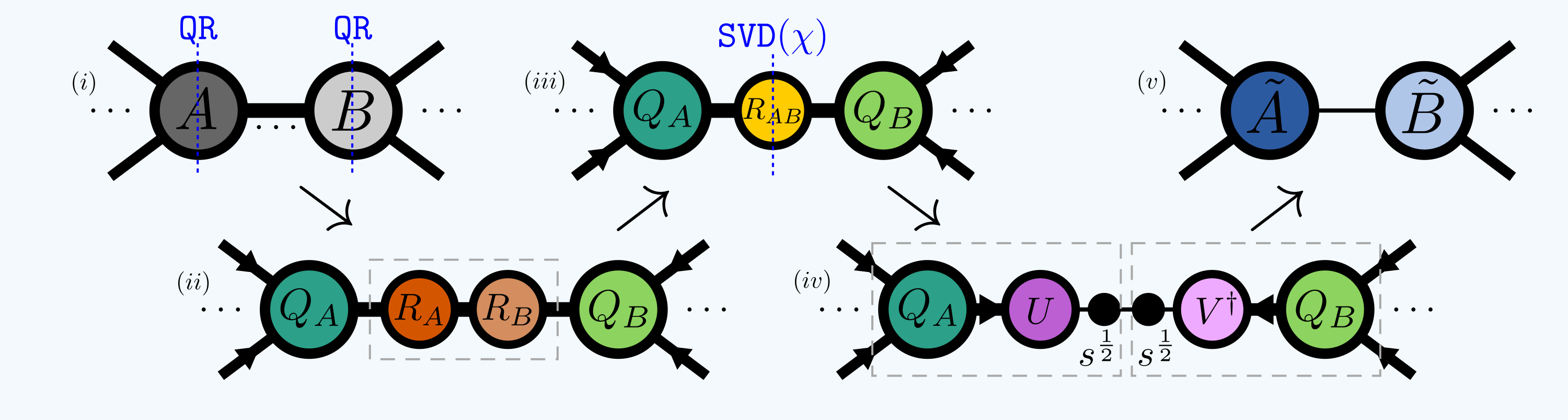
The maximum bond dimension kept is often denoted \(\chi\). The core function that handles this is qtn.tensor_compress_bond.

ta = qtn.rand_tensor([4, 4, 10], ['a', 'b', 'c'], 'A')
tb = qtn.rand_tensor([10, 4, 4, 4], ['c', 'd', 'e', 'f'], 'B')
(ta | tb).draw(['A', 'B'], figsize=(4, 4), show_inds='bond-size')

# perform the compression
qtn.tensor_compress_bond(ta, tb, max_bond=2, absorb='left')

# should now see the bond has been reduced in size to 2
(ta | tb).draw(['A', 'B'], figsize=(4, 4), show_inds='bond-size')

Again, there are many options for controlling the compression that can be found in tensor_compress_bond(), which in turn calls tensor_split() on the central factor.

In order to perform compressions in a tensor network based on tags, one can call compress_between(), which also has options for taking the environment into account and is one of the main drivers for 2D contraction for example.

1.5.3. TNLinearOperator

Tensor networks can represent very large multi-linear operators implicitly - these are often too large to form a dense representation of explicitly. However, many iterative algorithms exist that only require the action of this operator on a vector, and this can be cast as a contraction that is usually much cheaper.

Consider the following contrived TN with overall shape (1000, 1000, 1000, 1000), but which is evidently low rank:

ta = qtn.rand_tensor([1000, 2, 2], inds=['a', 'w', 'x'], tags='A')
tb = qtn.rand_tensor([1000, 2, 2], inds=['b', 'w', 'y'], tags='B')
tc = qtn.rand_tensor([1000, 2, 2], inds=['c', 'x', 'z'], tags='C')
td = qtn.rand_tensor([1000, 2, 2], inds=['d', 'y', 'z'], tags='D')
tn = (ta | tb | tc | td)
tn.draw(['A', 'B', 'C', 'D'], show_inds='all')

View this as a TNLinearOperator which is a subclass of a scipy.sparse.linalg.LinearOperator and so can be supplied anywhere they can:

tnlo = tn.aslinearoperator(['a', 'b'], ['c', 'd'])
tnlo

<1000000x1000000 TNLinearOperator with dtype=float64>

I.e. it maps a vector of size 1,000,000 spanning the indices 'a' and 'b' to a vector of size 1,000,000 spanning the indices 'c' and 'd'.

We can supply it to iterative functions directly:

qu.eigvals(tnlo, k=1, which='LM')

array([6425.04063216+0.j])

Or the function tensor_split() also accepts a TNLinearOperator instead of a Tensor.

tn_decomp = qtn.tensor_split(
    tnlo,
    left_inds=tnlo.left_inds,
    right_inds=tnlo.right_inds,
    # make sure we supply a iterative method
    method='svds',  # {'rsvd', 'isvd', 'eigs', ...}
    max_bond=4,
)

tn_decomp.draw(['A', 'B', 'C', 'D'], show_inds='bond-size')

Again, this operation can be performed within a TN based on tags using the method replace_with_svd(). Or you can treat an entire tensor network as an operator to be decomposed with split().

Warning

You are of course here still limited by the size of the left and right vector spaces, which while generally are square root the size of the dense operator, nonetheless grow exponentially in number of indices.

1.6. Selection

Many methods use tags to specify which tensors to operator on within a TN. This is often used in conjuction with a which kwarg specifying how to match the tags. The following illustrates the options for a 2D TN which has both rows and columns tagged:

tn = qtn.TN2D_rand(5, 5, D=4)

Get tensors which have all of the tags:

tn.select(tags=['X2', 'Y3'], which='all').add_tag('ALL')
tn.draw('ALL', figsize=(3, 3))

Get tensors which don’t have all of the tags:

tn.select(tags=['X2', 'Y3'], which='!all').add_tag('!ALL')
tn.draw('!ALL', figsize=(3, 3))

Get tensors which have any of the tags:

tn.select(tags=['X2', 'Y3'], which='any').add_tag('ANY')
tn.draw('ANY', figsize=(3, 3))

Get tensors which don’t have any of the tags:

tn.select(tags=['X2', 'Y3'], which='!any').add_tag('!ANY')
tn.draw('!ANY', figsize=(3, 3))

Several methods exist for returning the tagged tensors directly:

• TensorNetwork.select - get a tagged region as a tensor network

• TensorNetwork.select_tensors - get tagged tensors directly

• TensorNetwork.partition - partition into a two tensor networks

• TensorNetwork.partition_tensors - partition into two groups of tensors directly

• TensorNetwork.select_local - get a local region as a tensor network

Using the tn[tags] syntax is like calling tn.select_tensors(tags, which='all'):

tn['X2', 'Y3']

Tensor(shape=(4, 4, 4, 4), inds=[_d0324aAAABX, _d0324aAAABZ, _d0324aAAABa, _d0324aAAABR], tags={I2,3, X2, Y3, ALL, ANY}),

backend=numpy, dtype=float64, data=...

Although some special tensor networks also accept a lattice coordinate here as well:

tn[2, 3]

Tensor(shape=(4, 4, 4, 4), inds=[_d0324aAAABX, _d0324aAAABZ, _d0324aAAABa, _d0324aAAABR], tags={I2,3, X2, Y3, ALL, ANY}),

backend=numpy, dtype=float64, data=...

Hint

You can iterate over all tensors in a tensor network like so:

for t in tn:
    ...

Behind the scenes, tensors in a tensor network are stored using a unique tid - an integer denoting which node they are in the network. See Design for a more low level description.

1.6.1. Virtual vs Copies

An important concept when selecting tensors from tensor networks is whether the operation takes a copy of the tensors, or is simply viewing them ‘virtually’. In the examples above because select() defaults to virtual=True, when we modified the tensors by adding the tags ('ALL', '!ALL', 'ANY', '!ANY'), we are modifying the tensors in the original network too. Similarly, when we construct a tensor network like so:

tn = qtn.TensorNetwork([ta, tb, tc, td], virtual=True)

which is equivalent to

tn = (ta | tb | tc | td)

the new TN is viewing those tensors and so changes to them will affect tn and vice versa. Note this is not the default behaviour.

Warning

The underlying tensor arrays - t.data - are always assumed to be immutable and for efficiency are never copied by default in quimb.

1.7. Modification

Whilst many high level functions handle all the tensor modifications for you, at some point you will likely want to directly update, for example, the data in a Tensor. The low-level method for performing arbitrary changes to a tensors data, inds and tags is modify().

The reason that this is encapsulated thus, which is something to be aware of, is so that the tensor can let any tensor networks viewing it know of the changes. For example, often we want to iterate over tensors in a TN and change them on this atomic level, but not have to worry about the TN’s efficient maps which keep track of all the indices and tags going out of sync.

tn = qtn.TN_rand_reg(12, 3, 3, seed=42)
tn.draw()

# add a random dangling index to each tensor
for t in tn:
    t.new_ind(qtn.rand_uuid(), size=2)

tn.draw()

# the TN efficiently keeps track of all indices and tags still
tn.outer_inds()

('_d0324aAAACH',
 '_d0324aAAACI',
 '_d0324aAAACJ',
 '_d0324aAAACK',
 '_d0324aAAACL',
 '_d0324aAAACM',
 '_d0324aAAACN',
 '_d0324aAAACO',
 '_d0324aAAACP',
 '_d0324aAAACQ',
 '_d0324aAAACR',
 '_d0324aAAACS')

See the page Design for more details.