1. Basics

The quimb.operator module provides a unified way of ‘symbolically’ defining Hamiltonians or operators, including in symmetry sub-sectors, which can then be built into multiple different concrete representations for consumption by either the matrix or tensor network routines in quimb.

Matrix representations:

• Dense matrix

• Sparse matrix

• Linear operator (action on a dense vector)

Tensor network representations:

• Matrix product operator (MPO)

• Dict of local dense terms (for PEPS algorithms)

• Projected entangled pair operator (PEPO)

VMC routines:

• Coupled configurations

There is also support for certain transformations of the terms, such as the Jordan-Wigner transformation and pauli decomposition.

Here we’ll illustrate with a 2D Heisenberg model.

%config InlineBackend.figure_formats = ['svg']
import matplotlib as mpl
import matplotlib.pyplot as plt

import quimb as qu
import quimb.operator as qop
import quimb.tensor as qtn

mpl.style.use(qu.NEUTRAL_STYLE)

1.1. The HilbertSpace

For full control over the sites in our system and how to order them we first explicitly declare a HilbertSpace object, here for a 2D square lattice.

Lx = 4
Ly = 5
sites = [(i, j) for i in range(Lx) for j in range(Ly)]
nsites = len(sites)

# define a default symmetry sector for efficiency
symmetry = "U1"
sector = nsites // 2

hilbert_space = qop.HilbertSpace(
    sites=sites,
    symmetry=symmetry,
    sector=sector,
)
hilbert_space

HilbertSpace(nsites=20, total_size=184_756, symmetry=U1, sector=10)

On its own this just has a few helpful tools for enumerating the valid configurations. The terminology used here is:

• site: the labels of the individual sites in the system, these can be arbitrary hashable and sortable objects, e.g. our 2D coordinates above.

• reg: in a linear ordering of the sites, the reg is the integer index or ‘register’ of a site. This can be controlled using the order argument to the HilbertSpace constructor, which takes a sorting key, an explicit permutation, or one of the named presets described in the glossary below.

The ordering is fixed when the space is constructed, use with_ordering to get a new space ordered differently.

hilbert_space.site_to_reg((2, 3))

13

hilbert_space.reg_to_site(nsites - 1)

(3, 4)

Individual configurations can be referred to in three ways:

• config: a dict of site to local state.

• flatconfig: a numpy.ndarray[uint8] of local states in register order.

• rank: an integer between 0 and hilbert_space.size - 1 indexing the configurations in lexicographically sorted order.

# the first configuration (00..011..1) as a dict:
print(hilbert_space.rank_to_config(0))

{(0, 0): np.uint8(0), (0, 1): np.uint8(0), (0, 2): np.uint8(0), (0, 3): np.uint8(0), (0, 4): np.uint8(0), (1, 0): np.uint8(0), (1, 1): np.uint8(0), (1, 2): np.uint8(0), (1, 3): np.uint8(0), (1, 4): np.uint8(0), (2, 0): np.uint8(1), (2, 1): np.uint8(1), (2, 2): np.uint8(1), (2, 3): np.uint8(1), (2, 4): np.uint8(1), (3, 0): np.uint8(1), (3, 1): np.uint8(1), (3, 2): np.uint8(1), (3, 3): np.uint8(1), (3, 4): np.uint8(1)}

# get a random configuration
config = hilbert_space.rand_config(seed=42)
print(config)

{(0, 0): np.uint8(0), (0, 1): np.uint8(0), (0, 2): np.uint8(0), (0, 3): np.uint8(1), (0, 4): np.uint8(1), (1, 0): np.uint8(1), (1, 1): np.uint8(0), (1, 2): np.uint8(0), (1, 3): np.uint8(1), (1, 4): np.uint8(0), (2, 0): np.uint8(1), (2, 1): np.uint8(1), (2, 2): np.uint8(0), (2, 3): np.uint8(0), (2, 4): np.uint8(0), (3, 0): np.uint8(1), (3, 1): np.uint8(1), (3, 2): np.uint8(1), (3, 3): np.uint8(0), (3, 4): np.uint8(1)}

# find its rank
hilbert_space.config_to_rank(config)

16489

# the last configuration (11..100..0) as a flat vector
hilbert_space.rank_to_flatconfig(hilbert_space.size - 1)

array([1, 1, 1, 1, 1, 1, 1, 1, 1, 1, 0, 0, 0, 0, 0, 0, 0, 0, 0, 0],
      dtype=uint8)

1.2. The SparseOperatorBuilder

Now we can ‘symbolically’ define operators for this Hilbert space using the SparseOperatorBuilder object. Here we’ll define a 2D Heisenberg Hamiltonian:

H = qop.SparseOperatorBuilder(hilbert_space=hilbert_space)

# add nearest neighbor Heisenberg interactions
for i in range(Lx):
    for j in range(Ly):
        if i < Lx - 1:
            H += 0.5, ("+", (i, j)), ("-", (i + 1, j))
            H += 0.5, ("-", (i, j)), ("+", (i + 1, j))
            H += 1.0, ("z", (i, j)), ("z", (i + 1, j))
        if j < Ly - 1:
            H += 0.5, ("+", (i, j)), ("-", (i, j + 1))
            H += 0.5, ("-", (i, j)), ("+", (i, j + 1))
            H += 1.0, ("z", (i, j)), ("z", (i, j + 1))

# and a single site magnetic field to break symmetry
H += -0.1, ("z", (0, 0))

Note

If you don’t supply a HilbertSpace then the operator builder will build the default one for the minimal set of sites in has seen so far.

We can see all the terms visually with the show method (again the ordering is given by the register order):

H.show()

SparseOperatorBuilder(nsites=20, nterms=94, locality=2)
+ . . . . - . . . . . . . . . . . . . .  +0.5
- . . . . + . . . . . . . . . . . . . .  +0.5
z . . . . z . . . . . . . . . . . . . .  +1.0
+ - . . . . . . . . . . . . . . . . . .  +0.5
- + . . . . . . . . . . . . . . . . . .  +0.5
z z . . . . . . . . . . . . . . . . . .  +1.0
. + . . . . - . . . . . . . . . . . . .  +0.5
. - . . . . + . . . . . . . . . . . . .  +0.5
. z . . . . z . . . . . . . . . . . . .  +1.0
. + - . . . . . . . . . . . . . . . . .  +0.5
. - + . . . . . . . . . . . . . . . . .  +0.5
. z z . . . . . . . . . . . . . . . . .  +1.0
. . + . . . . - . . . . . . . . . . . .  +0.5
. . - . . . . + . . . . . . . . . . . .  +0.5
. . z . . . . z . . . . . . . . . . . .  +1.0
. . + - . . . . . . . . . . . . . . . .  +0.5
. . - + . . . . . . . . . . . . . . . .  +0.5
. . z z . . . . . . . . . . . . . . . .  +1.0
. . . + . . . . - . . . . . . . . . . .  +0.5
. . . - . . . . + . . . . . . . . . . .  +0.5
. . . z . . . . z . . . . . . . . . . .  +1.0
. . . + - . . . . . . . . . . . . . . .  +0.5
. . . - + . . . . . . . . . . . . . . .  +0.5
. . . z z . . . . . . . . . . . . . . .  +1.0
. . . . + . . . . - . . . . . . . . . .  +0.5
. . . . - . . . . + . . . . . . . . . .  +0.5
. . . . z . . . . z . . . . . . . . . .  +1.0
. . . . . + . . . . - . . . . . . . . .  +0.5
. . . . . - . . . . + . . . . . . . . .  +0.5
. . . . . z . . . . z . . . . . . . . .  +1.0
. . . . . + - . . . . . . . . . . . . .  +0.5
. . . . . - + . . . . . . . . . . . . .  +0.5
. . . . . z z . . . . . . . . . . . . .  +1.0
. . . . . . + . . . . - . . . . . . . .  +0.5
. . . . . . - . . . . + . . . . . . . .  +0.5
. . . . . . z . . . . z . . . . . . . .  +1.0
. . . . . . + - . . . . . . . . . . . .  +0.5
. . . . . . - + . . . . . . . . . . . .  +0.5
. . . . . . z z . . . . . . . . . . . .  +1.0
. . . . . . . + . . . . - . . . . . . .  +0.5
. . . . . . . - . . . . + . . . . . . .  +0.5
. . . . . . . z . . . . z . . . . . . .  +1.0
. . . . . . . + - . . . . . . . . . . .  +0.5
. . . . . . . - + . . . . . . . . . . .  +0.5
. . . . . . . z z . . . . . . . . . . .  +1.0
. . . . . . . . + . . . . - . . . . . .  +0.5
. . . . . . . . - . . . . + . . . . . .  +0.5
. . . . . . . . z . . . . z . . . . . .  +1.0
. . . . . . . . + - . . . . . . . . . .  +0.5
. . . . . . . . - + . . . . . . . . . .  +0.5
. . . . . . . . z z . . . . . . . . . .  +1.0
. . . . . . . . . + . . . . - . . . . .  +0.5
. . . . . . . . . - . . . . + . . . . .  +0.5
. . . . . . . . . z . . . . z . . . . .  +1.0
. . . . . . . . . . + . . . . - . . . .  +0.5
. . . . . . . . . . - . . . . + . . . .  +0.5
. . . . . . . . . . z . . . . z . . . .  +1.0
. . . . . . . . . . + - . . . . . . . .  +0.5
. . . . . . . . . . - + . . . . . . . .  +0.5
. . . . . . . . . . z z . . . . . . . .  +1.0
. . . . . . . . . . . + . . . . - . . .  +0.5
. . . . . . . . . . . - . . . . + . . .  +0.5
. . . . . . . . . . . z . . . . z . . .  +1.0
. . . . . . . . . . . + - . . . . . . .  +0.5
. . . . . . . . . . . - + . . . . . . .  +0.5
. . . . . . . . . . . z z . . . . . . .  +1.0
. . . . . . . . . . . . + . . . . - . .  +0.5
. . . . . . . . . . . . - . . . . + . .  +0.5
. . . . . . . . . . . . z . . . . z . .  +1.0
. . . . . . . . . . . . + - . . . . . .  +0.5
. . . . . . . . . . . . - + . . . . . .  +0.5
. . . . . . . . . . . . z z . . . . . .  +1.0
. . . . . . . . . . . . . + . . . . - .  +0.5
. . . . . . . . . . . . . - . . . . + .  +0.5
. . . . . . . . . . . . . z . . . . z .  +1.0
. . . . . . . . . . . . . + - . . . . .  +0.5
. . . . . . . . . . . . . - + . . . . .  +0.5
. . . . . . . . . . . . . z z . . . . .  +1.0
. . . . . . . . . . . . . . + . . . . -  +0.5
. . . . . . . . . . . . . . - . . . . +  +0.5
. . . . . . . . . . . . . . z . . . . z  +1.0
. . . . . . . . . . . . . . . + - . . .  +0.5
. . . . . . . . . . . . . . . - + . . .  +0.5
. . . . . . . . . . . . . . . z z . . .  +1.0
. . . . . . . . . . . . . . . . + - . .  +0.5
. . . . . . . . . . . . . . . . - + . .  +0.5
. . . . . . . . . . . . . . . . z z . .  +1.0
. . . . . . . . . . . . . . . . . + - .  +0.5
. . . . . . . . . . . . . . . . . - + .  +0.5
. . . . . . . . . . . . . . . . . z z .  +1.0
. . . . . . . . . . . . . . . . . . + -  +0.5
. . . . . . . . . . . . . . . . . . - +  +0.5
. . . . . . . . . . . . . . . . . . z z  +1.0
z . . . . . . . . . . . . . . . . . . .  -0.1

Currently the supported local operators are:

{
    "I": {0: (0, 1.0), 1: (1, 1.0)},
    # pauli matrices
    "x": {0: (1, 1.0), 1: (0, 1.0)},
    "y": {0: (1, 1.0j), 1: (0, -1.0j)},
    "z": {0: (0, 1.0), 1: (1, -1.0)},
    # ZX=iY: 'real Y'
    "⧖": {0: (1, -1.0), 1: (0, 1.0)},
    # spin 1/2 matrices (scaled paulis)
    "sx": {0: (1, 0.5), 1: (0, 0.5)},
    "sy": {0: (1, 0.5j), 1: (0, -0.5j)},
    "sz": {0: (0, 0.5), 1: (1, -0.5)},
    # creation / annihilation operators
    "+": {0: (1, 1.0)},
    "-": {1: (0, 1.0)},
    # number, symmetric number, and hole operators
    "n": {1: (1, 1.0)},
    "sn": {0: (0, -0.5), 1: (1, 0.5)},
    "h": {0: (0, 1.0)},
}

1.2.1. Building matrices

Now we can build out concrete realizations of the operator. For example the sparse matrix representation:

Hint

By default this will pick up the default sector and symmetry from the hilbert space object, or you can explicitly override it here.

%%time
H_sparse = H.build_sparse_matrix()
H_sparse

CPU times: user 992 ms, sys: 180 ms, total: 1.17 s
Wall time: 1.18 s

<Compressed Sparse Row sparse matrix of dtype 'float64'
	with 3199196 stored elements and shape (184756, 184756)>

This allows us to find the full exact groundstate and energy:

%%time
energy, psi = qu.eigh(H_sparse, k=1)

CPU times: user 5.01 s, sys: 82.5 ms, total: 5.09 s
Wall time: 694 ms

energy

array([-32.01392954])

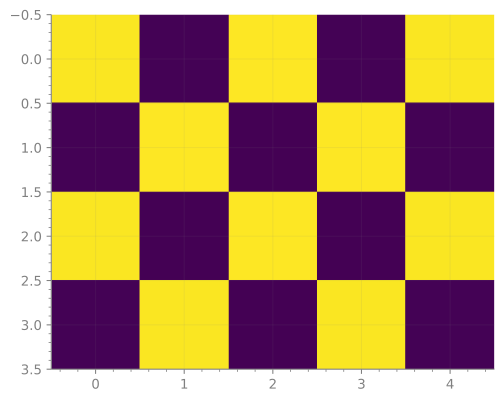
Now we can define some other operators that act on the same hilbert space, and measure their expectation, here the Z magnetization acting on every site:

zijs = [[None for j in range(Ly)] for i in range(Lx)]

for i in range(Lx):
    for j in range(Ly):
        zop_ij = qop.SparseOperatorBuilder(
            # we can supply all the terms at construction
            terms=[(1.0, ("z", (i, j)))],
            # because we only act on 1 site of many, we do
            # need to explicitly provide the hilbert space
            hilbert_space=hilbert_space,
        )

        # build the sparse matrix
        zsparse_ij = zop_ij.build_sparse_matrix()

        # evaluate <psi|Z_ij|psi>
        zijs[i][j] = qu.expec(psi, zsparse_ij)

plt.imshow(zijs)

<matplotlib.image.AxesImage at 0x731f57a8dfd0>

If this was a smaller space we could also build the full dense matrix with build_dense.

The SparseOperatorBuilder also has a matvec method which computes the action on a dense vector without forming the explicit matrix. You can use this directly or call .aslinearoperator to get a scipy.sparse.linalg.LinearOperator object which can be used with scipy.sparse.linalg routines.

Warning

This is not a very efficient implementation yet, you may want to consider for example quspin if performance is critical.

1.2.2. Building tensor network representations

1.2.2.1. Building MPOs for MPS algorithms

We can also build out concrete representations of the operator for consumption by various tensor network algorithms in quimb.tensor.

For example as a matrix product operator (MPO) using build_mpo:

H_mpo = H.build_mpo()
H_mpo

MatrixProductOperator(tensors=20, indices=59, L=20, max_bond=17)

Tensor(shape=(4, 2, 2), inds=[_23d24bAAAAB, k0, b0], tags={I0}),

backend=numpy, dtype=float64, data=array([[[ 0., 0.], [ 1., 0.]], [[ 0., 1.], [ 0., 0.]], [[ 1., 0.], [ 0., -1.]], [[ 1., 0.], [ 0., 1.]]])

Tensor(shape=(4, 8, 2, 2), inds=[_23d24bAAAAB, _23d24bAAAAC, k1, b1], tags={I1}),

backend=numpy, dtype=float64, data=...

Tensor(shape=(8, 11, 2, 2), inds=[_23d24bAAAAC, _23d24bAAAAD, k2, b2], tags={I2}),

backend=numpy, dtype=float64, data=...

Tensor(shape=(11, 14, 2, 2), inds=[_23d24bAAAAD, _23d24bAAAAE, k3, b3], tags={I3}),

backend=numpy, dtype=float64, data=...

Tensor(shape=(14, 17, 2, 2), inds=[_23d24bAAAAE, _23d24bAAAAF, k4, b4], tags={I4}),

backend=numpy, dtype=float64, data=...

Tensor(shape=(17, 17, 2, 2), inds=[_23d24bAAAAF, _23d24bAAAAG, k5, b5], tags={I5}),

backend=numpy, dtype=float64, data=...

Tensor(shape=(17, 17, 2, 2), inds=[_23d24bAAAAG, _23d24bAAAAH, k6, b6], tags={I6}),

backend=numpy, dtype=float64, data=...

Tensor(shape=(17, 17, 2, 2), inds=[_23d24bAAAAH, _23d24bAAAAI, k7, b7], tags={I7}),

backend=numpy, dtype=float64, data=...

Tensor(shape=(17, 17, 2, 2), inds=[_23d24bAAAAI, _23d24bAAAAJ, k8, b8], tags={I8}),

backend=numpy, dtype=float64, data=...

Tensor(shape=(17, 17, 2, 2), inds=[_23d24bAAAAJ, _23d24bAAAAK, k9, b9], tags={I9}),

backend=numpy, dtype=float64, data=...

Tensor(shape=(17, 17, 2, 2), inds=[_23d24bAAAAK, _23d24bAAAAL, k10, b10], tags={I10}),

backend=numpy, dtype=float64, data=...

Tensor(shape=(17, 17, 2, 2), inds=[_23d24bAAAAL, _23d24bAAAAM, k11, b11], tags={I11}),

backend=numpy, dtype=float64, data=...

Tensor(shape=(17, 17, 2, 2), inds=[_23d24bAAAAM, _23d24bAAAAN, k12, b12], tags={I12}),

backend=numpy, dtype=float64, data=...

Tensor(shape=(17, 17, 2, 2), inds=[_23d24bAAAAN, _23d24bAAAAO, k13, b13], tags={I13}),

backend=numpy, dtype=float64, data=...

Tensor(shape=(17, 17, 2, 2), inds=[_23d24bAAAAO, _23d24bAAAAP, k14, b14], tags={I14}),

backend=numpy, dtype=float64, data=...

Tensor(shape=(17, 14, 2, 2), inds=[_23d24bAAAAP, _23d24bAAAAQ, k15, b15], tags={I15}),

backend=numpy, dtype=float64, data=...

Tensor(shape=(14, 11, 2, 2), inds=[_23d24bAAAAQ, _23d24bAAAAR, k16, b16], tags={I16}),

backend=numpy, dtype=float64, data=...

Tensor(shape=(11, 8, 2, 2), inds=[_23d24bAAAAR, _23d24bAAAAS, k17, b17], tags={I17}),

backend=numpy, dtype=float64, data=...

Tensor(shape=(8, 4, 2, 2), inds=[_23d24bAAAAS, _23d24bAAAAT, k18, b18], tags={I18}),

backend=numpy, dtype=float64, data=...

Tensor(shape=(4, 2, 2), inds=[_23d24bAAAAT, k19, b19], tags={I19}),

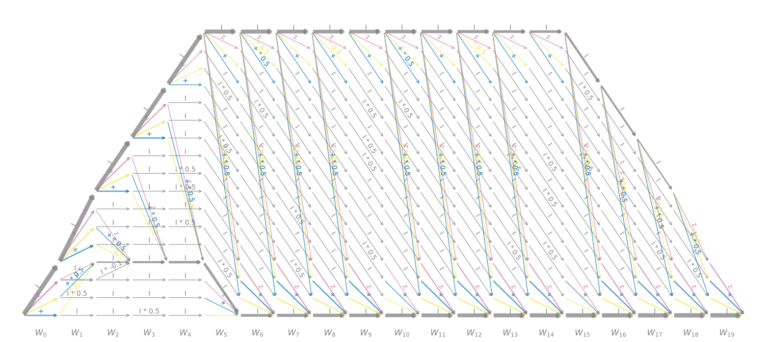
backend=numpy, dtype=float64, data=array([[[ 1., 0.], [ 0., 1.]], [[ 0., 1.], [ 0., 0.]], [[ 0., 0.], [ 1., 0.]], [[ 1., 0.], [ 0., -1.]]])

The algorithm to build the MPO is a greedy algorithm that works well for local Hamiltonians, but will not be optimal for complicated long range models. You can check the underyling finite state machine representatino with draw_state_machine:

H.draw_state_machine()

We can use the MPO to find the groundstate with DMRG:

dmrg = qtn.DMRG2(H_mpo)
dmrg.solve(verbosity=1)

1, R, max_bond=(8/8), cutoff:1e-08

100%|##########################################| 19/19 [00:00<00:00, 306.08it/s]

Energy: -31.656832428772546 ... not converged.
2, R, max_bond=(8/16), cutoff:1e-08

100%|##########################################| 19/19 [00:00<00:00, 362.23it/s]

Energy: -31.813407135272556 ... not converged.
3, R, max_bond=(16/32), cutoff:1e-08

100%|##########################################| 19/19 [00:00<00:00, 279.30it/s]

Energy: -31.818448856710024 ... not converged.
4, R, max_bond=(29/64), cutoff:1e-08

100%|##########################################| 19/19 [00:00<00:00, 192.93it/s]

Energy: -31.81932769634487 ... not converged.
5, R, max_bond=(39/128), cutoff:1e-08

100%|##########################################| 19/19 [00:00<00:00, 152.65it/s]

Energy: -31.81949636476171 ... not converged.
6, R, max_bond=(42/256), cutoff:1e-08

100%|##########################################| 19/19 [00:00<00:00, 210.71it/s]

Energy: -31.819509858329468 ... converged!

np.True_

Then we can check the relative error in the groundstate energy:

1 - dmrg.energy / energy.item()

np.float64(0.006072971495561852)

1.2.2.2. Building local terms for PEPS

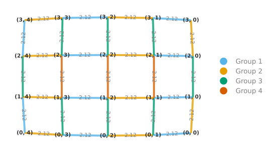
For projected entangled pair states (PEPS) algorithms we often need the local terms of the Hamiltonian as dense matrices. We can build these with build_local_ham:

H_local = H.build_local_ham()
H_local.draw()

(<Figure size 547.214x547.214 with 1 Axes>, <Axes: >)

We can then feed this into algorithms such as simple update:

peps = qtn.PEPS.rand(Lx, Ly, 4, seed=42)
su = qtn.SimpleUpdate(peps, H_local)
su.evolve(100, tau=0.1)

n=100, D=4, tau=0.1, energy≈-31.9678: 100%|##########| 100/100 [00:02<00:00, 35.70it/s]

1 - su.energy / energy.item()

0.0014423055073261581

1.2.3. Monte carlo usage

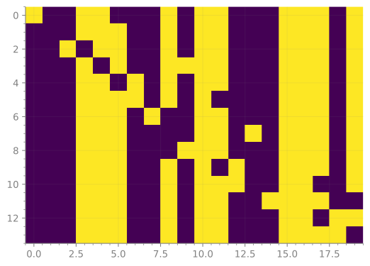
For variational monte carlo (VMC) or other monte carlo routines one needs to the compute the ‘local energy’. This is encapsulated in the config_coupling and flatconfig_coupling methods. These return a tuple with A) the coupled configurations and B) the corresponding coefficients.

Mathematically, for a given configuration \(| x \rangle\), this returns the non-zero coupled configurations: \(\{| y \rangle\} \), as well as the coefficients \(\{ \langle x | H | y \rangle \}\) such that the ‘local energy’ is given by:

\[ E_{\text{loc}}(x) = \sum_y \dfrac{ \langle x | H | y \rangle \langle y | \psi \rangle } { \langle x | \psi \rangle } \]

flatconfig = hilbert_space.rand_flatconfig(seed=42)
flatconfig

array([0, 0, 0, 1, 1, 1, 0, 0, 1, 0, 1, 1, 0, 0, 0, 1, 1, 1, 0, 1],
      dtype=uint8)

coupled_flatconfigs, coupled_coeffs = H.flatconfig_coupling(flatconfig)
coupled_flatconfigs, coupled_coeffs

(array([[1, 0, 0, 1, 1, 0, 0, 0, 1, 0, 1, 1, 0, 0, 0, 1, 1, 1, 0, 1],
        [0, 0, 0, 1, 1, 1, 0, 0, 1, 0, 1, 1, 0, 0, 0, 1, 1, 1, 0, 1],
        [0, 0, 1, 0, 1, 1, 0, 0, 1, 0, 1, 1, 0, 0, 0, 1, 1, 1, 0, 1],
        [0, 0, 0, 1, 0, 1, 0, 0, 1, 1, 1, 1, 0, 0, 0, 1, 1, 1, 0, 1],
        [0, 0, 0, 1, 1, 0, 1, 0, 1, 0, 1, 1, 0, 0, 0, 1, 1, 1, 0, 1],
        [0, 0, 0, 1, 1, 1, 1, 0, 1, 0, 1, 0, 0, 0, 0, 1, 1, 1, 0, 1],
        [0, 0, 0, 1, 1, 1, 0, 1, 0, 0, 1, 1, 0, 0, 0, 1, 1, 1, 0, 1],
        [0, 0, 0, 1, 1, 1, 0, 0, 0, 0, 1, 1, 0, 1, 0, 1, 1, 1, 0, 1],
        [0, 0, 0, 1, 1, 1, 0, 0, 0, 1, 1, 1, 0, 0, 0, 1, 1, 1, 0, 1],
        [0, 0, 0, 1, 1, 1, 0, 0, 1, 0, 1, 0, 1, 0, 0, 1, 1, 1, 0, 1],
        [0, 0, 0, 1, 1, 1, 0, 0, 1, 0, 1, 1, 1, 0, 0, 1, 1, 0, 0, 1],
        [0, 0, 0, 1, 1, 1, 0, 0, 1, 0, 1, 1, 0, 0, 1, 1, 1, 1, 0, 0],
        [0, 0, 0, 1, 1, 1, 0, 0, 1, 0, 1, 1, 0, 0, 0, 1, 1, 0, 1, 1],
        [0, 0, 0, 1, 1, 1, 0, 0, 1, 0, 1, 1, 0, 0, 0, 1, 1, 1, 1, 0]],
       dtype=uint8),
 array([0.5, 4.9, 0.5, 0.5, 0.5, 0.5, 0.5, 0.5, 0.5, 0.5, 0.5, 0.5, 0.5,
        0.5]))

plt.imshow(coupled_flatconfigs)

<matplotlib.image.AxesImage at 0x731f54488050>

1.2.4. Transforming operators

The SparseOperatorBuilder also has some methods for transforming the terms.

1.2.4.1. Jordan-Wigner transformation

For example the Jordan-Wigner transformation which maps spin-1/2 operators to fermionic ones:

Here the sites carry a spin label as well as a coordinate, so we tell the HilbertSpace which species each site belongs to. That lets the filling of each be given directly, and is what lets a U1U1 sector be used with any ordering.

Note

The order matters for fermions: it fixes where the Jordan-Wigner Z strings go. "blocked" puts all of one spin then all of the other, so the strings stay within a spin species. "interleaved" alternates them, which adds one Z per hopping term but makes the on-site interaction register local, giving a much smaller MPO. The latter is the default for fermi_hubbard_from_edges.

Lx = 4
Ly = 3
sites = [(s, i, j) for s in ("u", "d") for i in range(Lx) for j in range(Ly)]
nsites = len(sites)

# define half filling in each species
symmetry = "U1U1"
sector = {"u": nsites // 4, "d": nsites // 4}

hilbert_space = qop.HilbertSpace(
    sites=sites,
    # the first label of each site says which species it is
    species=lambda site: site[0],
    symmetry=symmetry,
    sector=sector,
)
hilbert_space

HilbertSpace(nsites=24, total_size=853_776, symmetry=U1U1, sector=((12, 6), (12, 6)))

H = qop.SparseOperatorBuilder(hilbert_space=hilbert_space)

t = 1.0
U = 8.0

# add nearest neighbor Heisenberg interactions
for i in range(Lx):
    for j in range(Ly):
        for s in ("u", "d"):
            # hopping
            if i < Lx - 1:
                # the relative ordering within the term now matters too
                H.add_term(-t, ("+", (s, i, j)), ("-", (s, i + 1, j)))
                H.add_term(-t, ("+", (s, i + 1, j)), ("-", (s, i, j)))
            if j < Ly - 1:
                H.add_term(-t, ("+", (s, i, j)), ("-", (s, i, j + 1)))
                H.add_term(-t, ("+", (s, i, j + 1)), ("-", (s, i, j)))

        # interaction
        H.add_term(U, ("n", ("u", i, j)), ("n", ("d", i, j)))

Note

You can either call the method jordan_wigner_transform to toggle the transformation, or supply jordan_wigner=True to the SparseOperatorBuilder constructor.

H.jordan_wigner_transform()
H.show()

SparseOperatorBuilder(nsites=24, nterms=80, locality=4, jordan_wigner=True)
+ z z - . . . . . . . . . . . . . . . . . . . .  -1.0
- z z + . . . . . . . . . . . . . . . . . . . .  -1.0
+ - . . . . . . . . . . . . . . . . . . . . . .  -1.0
- + . . . . . . . . . . . . . . . . . . . . . .  -1.0
. . . . . . . . . . . . + z z - . . . . . . . .  -1.0
. . . . . . . . . . . . - z z + . . . . . . . .  -1.0
. . . . . . . . . . . . + - . . . . . . . . . .  -1.0
. . . . . . . . . . . . - + . . . . . . . . . .  -1.0
n . . . . . . . . . . . n . . . . . . . . . . .  +8.0
. + z z - . . . . . . . . . . . . . . . . . . .  -1.0
. - z z + . . . . . . . . . . . . . . . . . . .  -1.0
. + - . . . . . . . . . . . . . . . . . . . . .  -1.0
. - + . . . . . . . . . . . . . . . . . . . . .  -1.0
. . . . . . . . . . . . . + z z - . . . . . . .  -1.0
. . . . . . . . . . . . . - z z + . . . . . . .  -1.0
. . . . . . . . . . . . . + - . . . . . . . . .  -1.0
. . . . . . . . . . . . . - + . . . . . . . . .  -1.0
. n . . . . . . . . . . . n . . . . . . . . . .  +8.0
. . + z z - . . . . . . . . . . . . . . . . . .  -1.0
. . - z z + . . . . . . . . . . . . . . . . . .  -1.0
. . . . . . . . . . . . . . + z z - . . . . . .  -1.0
. . . . . . . . . . . . . . - z z + . . . . . .  -1.0
. . n . . . . . . . . . . . n . . . . . . . . .  +8.0
. . . + z z - . . . . . . . . . . . . . . . . .  -1.0
. . . - z z + . . . . . . . . . . . . . . . . .  -1.0
. . . + - . . . . . . . . . . . . . . . . . . .  -1.0
. . . - + . . . . . . . . . . . . . . . . . . .  -1.0
. . . . . . . . . . . . . . . + z z - . . . . .  -1.0
. . . . . . . . . . . . . . . - z z + . . . . .  -1.0
. . . . . . . . . . . . . . . + - . . . . . . .  -1.0
. . . . . . . . . . . . . . . - + . . . . . . .  -1.0
. . . n . . . . . . . . . . . n . . . . . . . .  +8.0
. . . . + z z - . . . . . . . . . . . . . . . .  -1.0
. . . . - z z + . . . . . . . . . . . . . . . .  -1.0
. . . . + - . . . . . . . . . . . . . . . . . .  -1.0
. . . . - + . . . . . . . . . . . . . . . . . .  -1.0
. . . . . . . . . . . . . . . . + z z - . . . .  -1.0
. . . . . . . . . . . . . . . . - z z + . . . .  -1.0
. . . . . . . . . . . . . . . . + - . . . . . .  -1.0
. . . . . . . . . . . . . . . . - + . . . . . .  -1.0
. . . . n . . . . . . . . . . . n . . . . . . .  +8.0
. . . . . + z z - . . . . . . . . . . . . . . .  -1.0
. . . . . - z z + . . . . . . . . . . . . . . .  -1.0
. . . . . . . . . . . . . . . . . + z z - . . .  -1.0
. . . . . . . . . . . . . . . . . - z z + . . .  -1.0
. . . . . n . . . . . . . . . . . n . . . . . .  +8.0
. . . . . . + z z - . . . . . . . . . . . . . .  -1.0
. . . . . . - z z + . . . . . . . . . . . . . .  -1.0
. . . . . . + - . . . . . . . . . . . . . . . .  -1.0
. . . . . . - + . . . . . . . . . . . . . . . .  -1.0
. . . . . . . . . . . . . . . . . . + z z - . .  -1.0
. . . . . . . . . . . . . . . . . . - z z + . .  -1.0
. . . . . . . . . . . . . . . . . . + - . . . .  -1.0
. . . . . . . . . . . . . . . . . . - + . . . .  -1.0
. . . . . . n . . . . . . . . . . . n . . . . .  +8.0
. . . . . . . + z z - . . . . . . . . . . . . .  -1.0
. . . . . . . - z z + . . . . . . . . . . . . .  -1.0
. . . . . . . + - . . . . . . . . . . . . . . .  -1.0
. . . . . . . - + . . . . . . . . . . . . . . .  -1.0
. . . . . . . . . . . . . . . . . . . + z z - .  -1.0
. . . . . . . . . . . . . . . . . . . - z z + .  -1.0
. . . . . . . . . . . . . . . . . . . + - . . .  -1.0
. . . . . . . . . . . . . . . . . . . - + . . .  -1.0
. . . . . . . n . . . . . . . . . . . n . . . .  +8.0
. . . . . . . . + z z - . . . . . . . . . . . .  -1.0
. . . . . . . . - z z + . . . . . . . . . . . .  -1.0
. . . . . . . . . . . . . . . . . . . . + z z -  -1.0
. . . . . . . . . . . . . . . . . . . . - z z +  -1.0
. . . . . . . . n . . . . . . . . . . . n . . .  +8.0
. . . . . . . . . + - . . . . . . . . . . . . .  -1.0
. . . . . . . . . - + . . . . . . . . . . . . .  -1.0
. . . . . . . . . . . . . . . . . . . . . + - .  -1.0
. . . . . . . . . . . . . . . . . . . . . - + .  -1.0
. . . . . . . . . n . . . . . . . . . . . n . .  +8.0
. . . . . . . . . . + - . . . . . . . . . . . .  -1.0
. . . . . . . . . . - + . . . . . . . . . . . .  -1.0
. . . . . . . . . . . . . . . . . . . . . . + -  -1.0
. . . . . . . . . . . . . . . . . . . . . . - +  -1.0
. . . . . . . . . . n . . . . . . . . . . . n .  +8.0
. . . . . . . . . . . n . . . . . . . . . . . n  +8.0

H_sparse = H.build_sparse_matrix()
H_sparse

<Compressed Sparse Row sparse matrix of dtype 'float64'
	with 16686516 stored elements and shape (853776, 853776)>

energy, psi = qu.eigh(H_sparse, k=1)
energy / (Lx * Ly)

array([-0.40943827])

1.2.4.2. Pauli Decomposition

You can also decompose an operator into strings of Pauli operators using the pauli_decompose method, or by supplying pauli_decompose=True to the SparseOperatorBuilder constructor. The use_zx argument enables decomposing Y operators into the real combination of Z and X (i.e. ⴵ = ZX = iY) to avoid complex coefficients:

H.pauli_decompose(use_zx=True)
H.show()

SparseOperatorBuilder(nsites=24, nterms=105, locality=4, jordan_wigner=True, pauli_decompose=zx)
x z z x . . . . . . . . . . . . . . . . . . . .  -0.5
ⴵ z z ⴵ . . . . . . . . . . . . . . . . . . . .  +0.5
x x . . . . . . . . . . . . . . . . . . . . . .  -0.5
ⴵ ⴵ . . . . . . . . . . . . . . . . . . . . . .  +0.5
. . . . . . . . . . . . x z z x . . . . . . . .  -0.5
. . . . . . . . . . . . ⴵ z z ⴵ . . . . . . . .  +0.5
. . . . . . . . . . . . x x . . . . . . . . . .  -0.5
. . . . . . . . . . . . ⴵ ⴵ . . . . . . . . . .  +0.5
z . . . . . . . . . . . . . . . . . . . . . . .  -2.0
. . . . . . . . . . . . z . . . . . . . . . . .  -2.0
z . . . . . . . . . . . z . . . . . . . . . . .  +2.0
. x z z x . . . . . . . . . . . . . . . . . . .  -0.5
. ⴵ z z ⴵ . . . . . . . . . . . . . . . . . . .  +0.5
. x x . . . . . . . . . . . . . . . . . . . . .  -0.5
. ⴵ ⴵ . . . . . . . . . . . . . . . . . . . . .  +0.5
. . . . . . . . . . . . . x z z x . . . . . . .  -0.5
. . . . . . . . . . . . . ⴵ z z ⴵ . . . . . . .  +0.5
. . . . . . . . . . . . . x x . . . . . . . . .  -0.5
. . . . . . . . . . . . . ⴵ ⴵ . . . . . . . . .  +0.5
. z . . . . . . . . . . . . . . . . . . . . . .  -2.0
. . . . . . . . . . . . . z . . . . . . . . . .  -2.0
. z . . . . . . . . . . . z . . . . . . . . . .  +2.0
. . x z z x . . . . . . . . . . . . . . . . . .  -0.5
. . ⴵ z z ⴵ . . . . . . . . . . . . . . . . . .  +0.5
. . . . . . . . . . . . . . x z z x . . . . . .  -0.5
. . . . . . . . . . . . . . ⴵ z z ⴵ . . . . . .  +0.5
. . z . . . . . . . . . . . . . . . . . . . . .  -2.0
. . . . . . . . . . . . . . z . . . . . . . . .  -2.0
. . z . . . . . . . . . . . z . . . . . . . . .  +2.0
. . . x z z x . . . . . . . . . . . . . . . . .  -0.5
. . . ⴵ z z ⴵ . . . . . . . . . . . . . . . . .  +0.5
. . . x x . . . . . . . . . . . . . . . . . . .  -0.5
. . . ⴵ ⴵ . . . . . . . . . . . . . . . . . . .  +0.5
. . . . . . . . . . . . . . . x z z x . . . . .  -0.5
. . . . . . . . . . . . . . . ⴵ z z ⴵ . . . . .  +0.5
. . . . . . . . . . . . . . . x x . . . . . . .  -0.5
. . . . . . . . . . . . . . . ⴵ ⴵ . . . . . . .  +0.5
. . . z . . . . . . . . . . . . . . . . . . . .  -2.0
. . . . . . . . . . . . . . . z . . . . . . . .  -2.0
. . . z . . . . . . . . . . . z . . . . . . . .  +2.0
. . . . x z z x . . . . . . . . . . . . . . . .  -0.5
. . . . ⴵ z z ⴵ . . . . . . . . . . . . . . . .  +0.5
. . . . x x . . . . . . . . . . . . . . . . . .  -0.5
. . . . ⴵ ⴵ . . . . . . . . . . . . . . . . . .  +0.5
. . . . . . . . . . . . . . . . x z z x . . . .  -0.5
. . . . . . . . . . . . . . . . ⴵ z z ⴵ . . . .  +0.5
. . . . . . . . . . . . . . . . x x . . . . . .  -0.5
. . . . . . . . . . . . . . . . ⴵ ⴵ . . . . . .  +0.5
. . . . z . . . . . . . . . . . . . . . . . . .  -2.0
. . . . . . . . . . . . . . . . z . . . . . . .  -2.0
. . . . z . . . . . . . . . . . z . . . . . . .  +2.0
. . . . . x z z x . . . . . . . . . . . . . . .  -0.5
. . . . . ⴵ z z ⴵ . . . . . . . . . . . . . . .  +0.5
. . . . . . . . . . . . . . . . . x z z x . . .  -0.5
. . . . . . . . . . . . . . . . . ⴵ z z ⴵ . . .  +0.5
. . . . . z . . . . . . . . . . . . . . . . . .  -2.0
. . . . . . . . . . . . . . . . . z . . . . . .  -2.0
. . . . . z . . . . . . . . . . . z . . . . . .  +2.0
. . . . . . x z z x . . . . . . . . . . . . . .  -0.5
. . . . . . ⴵ z z ⴵ . . . . . . . . . . . . . .  +0.5
. . . . . . x x . . . . . . . . . . . . . . . .  -0.5
. . . . . . ⴵ ⴵ . . . . . . . . . . . . . . . .  +0.5
. . . . . . . . . . . . . . . . . . x z z x . .  -0.5
. . . . . . . . . . . . . . . . . . ⴵ z z ⴵ . .  +0.5
. . . . . . . . . . . . . . . . . . x x . . . .  -0.5
. . . . . . . . . . . . . . . . . . ⴵ ⴵ . . . .  +0.5
. . . . . . z . . . . . . . . . . . . . . . . .  -2.0
. . . . . . . . . . . . . . . . . . z . . . . .  -2.0
. . . . . . z . . . . . . . . . . . z . . . . .  +2.0
. . . . . . . x z z x . . . . . . . . . . . . .  -0.5
. . . . . . . ⴵ z z ⴵ . . . . . . . . . . . . .  +0.5
. . . . . . . x x . . . . . . . . . . . . . . .  -0.5
. . . . . . . ⴵ ⴵ . . . . . . . . . . . . . . .  +0.5
. . . . . . . . . . . . . . . . . . . x z z x .  -0.5
. . . . . . . . . . . . . . . . . . . ⴵ z z ⴵ .  +0.5
. . . . . . . . . . . . . . . . . . . x x . . .  -0.5
. . . . . . . . . . . . . . . . . . . ⴵ ⴵ . . .  +0.5
. . . . . . . z . . . . . . . . . . . . . . . .  -2.0
. . . . . . . . . . . . . . . . . . . z . . . .  -2.0
. . . . . . . z . . . . . . . . . . . z . . . .  +2.0
. . . . . . . . x z z x . . . . . . . . . . . .  -0.5
. . . . . . . . ⴵ z z ⴵ . . . . . . . . . . . .  +0.5
. . . . . . . . . . . . . . . . . . . . x z z x  -0.5
. . . . . . . . . . . . . . . . . . . . ⴵ z z ⴵ  +0.5
. . . . . . . . z . . . . . . . . . . . . . . .  -2.0
. . . . . . . . . . . . . . . . . . . . z . . .  -2.0
. . . . . . . . z . . . . . . . . . . . z . . .  +2.0
. . . . . . . . . x x . . . . . . . . . . . . .  -0.5
. . . . . . . . . ⴵ ⴵ . . . . . . . . . . . . .  +0.5
. . . . . . . . . . . . . . . . . . . . . x x .  -0.5
. . . . . . . . . . . . . . . . . . . . . ⴵ ⴵ .  +0.5
. . . . . . . . . z . . . . . . . . . . . . . .  -2.0
. . . . . . . . . . . . . . . . . . . . . z . .  -2.0
. . . . . . . . . z . . . . . . . . . . . z . .  +2.0
. . . . . . . . . . x x . . . . . . . . . . . .  -0.5
. . . . . . . . . . ⴵ ⴵ . . . . . . . . . . . .  +0.5
. . . . . . . . . . . . . . . . . . . . . . x x  -0.5
. . . . . . . . . . . . . . . . . . . . . . ⴵ ⴵ  +0.5
. . . . . . . . . . z . . . . . . . . . . . . .  -2.0
. . . . . . . . . . . . . . . . . . . . . . z .  -2.0
. . . . . . . . . . z . . . . . . . . . . . z .  +2.0
. . . . . . . . . . . . . . . . . . . . . . . .  +24.0
. . . . . . . . . . . z . . . . . . . . . . . .  -2.0
. . . . . . . . . . . . . . . . . . . . . . . z  -2.0
. . . . . . . . . . . z . . . . . . . . . . . z  +2.0

1.2.5. Builtin operators

The following hamiltonians are built in:

• heisenberg_from_edges: the Heisenberg model on an arbitrary graph defined by edges, includes the transverse field ising model as a special case of the coupling and magnetic field terms.

• fermi_hubbard_from_edges: the Fermi-Hubbard model on an arbitrary graph defined by edges.

• fermi_hubbard_spinless_from_edges: the spinless Fermi-Hubbard model (aka t-V model) on an arbitrary graph defined by edges.

1.2.6. Glossary

site

The label of a single site, any hashable and sortable object, such as the 2D coordinates used above. Terms are always written in terms of sites, never registers.

register

The integer index of a site in the linear ordering of the Hilbert space, from 0 to nsites - 1. Convert with site_to_reg and reg_to_site.

ordering

Which site gets which register, set by the order argument. This accepts a sorting key, an explicit permutation of the sites, True to sort them, or one of two presets for sites labelled (species, ...): "blocked" groups the sites into one contiguous block per species, "interleaved" alternates the species at each position. It is fixed at construction, see with_ordering. The choice matters because it sets where the Jordan-Wigner strings go and how local the terms are for MPO construction.

species

Which conserved charge a site’s occupation counts towards, e.g. spin up or down. Supplied as the species argument, either a function of the site or a mapping from site to label, and required for the shorter U1U1 sector forms.

config

A dict mapping each site to its local state.

flatconfig

A numpy.ndarray[uint8] of local states, in register order. Everything public that takes or returns a flatconfig uses this ordering, including flatconfig_coupling.

rank

An integer from 0 to hilbert_space.size - 1 indexing the valid configurations of the current symmetry and sector.

symmetry

The conserved quantity restricting which configurations are valid: None, "Z2", "U1", or "U1U1". Usually inferred from the sector.

sector

Which sector of that symmetry to work in: a parity for Z2, a filling for U1, and for U1U1 the filling of each species, written either as {species: filling}, as (ka, kb) paired with the species in sorted label order, or explicitly as ((na, ka), (nb, kb)). The first two need species to be supplied. A sector can also be given per call to the build methods, overriding the default one.

blocked ordering

The ordering that groups each species into one contiguous block, i.e. what the "blocked" preset produces. U1U1 always enumerates configurations in this ordering, whatever the registers are, so the two coincide unless the species are interleaved. Configurations crossing the public API are always in register order, so this surfaces only through site_to_blocked_reg.