3. MPI Interior Eigensolve with Lazy, Projected Operators

This example demonstrates some ‘advanced’ methods for diagonalizing large Hamiltonians.

First of all, assuming we are using slepc4py, we can specify the ‘arch’ we want to use. In this case, there is an optimized version of ‘petsc’ and ‘slepc’, compiled with float scalars, named 'arch-auto-real':

# optional - comment or ignore this cell to use the default arch
#     or specify your own arch
import os
os.environ['PETSC_ARCH'] = 'arch-auto-real'

For real problems (like below) this generally gives a bit of a speed boost. After doing that we can import quimb:

import quimb as qu

We are not going to contsruct the Hamiltonian directly, instead leave it as a Lazy object, so that each MPI process can construct its own rows and avoid redudant communication and memory. To do that we need to know the size of the matrix first:

# total hilbert space for 18 spin-1/2s
n = 18
d = 2**n
shape = (d, d)

# And make the lazy representation
H_opts = {'n': n, 'dh': 3.0, 'sparse': True, 'seed': 9}
H = qu.Lazy(qu.ham_mbl, **H_opts, shape=shape)
H

<Lazy(ham_mbl, shape=(262144, 262144))>

This Hamiltonian also conserves z-spin, which we can use to make the effective problem significantly smaller. This is done by supplying a projector onto the subspace we are targeting. We also need to know its size first if we want to leave it ‘unconstructed’:

# total Sz=0 subspace size (n choose n / 2)
from scipy.special import comb

ds = comb(n, n // 2, exact=True)
shape = (d, ds)

# And make the lazy representation
P = qu.Lazy(qu.zspin_projector, n=n, shape=shape)
P

<Lazy(zspin_projector, shape=(262144, 48620))>

Now we can solve the hamiltoniain, for 5 eigenpairs centered around energy 0:

%%time
lk, vk = qu.eigh(H, P=P, k=5, sigma=0.0, backend='slepc')
print('energies:', lk)

energies: [-9.10482079e-04 -7.21481890e-04 -2.40962026e-04 -1.77843488e-04
 -5.45274570e-05]
CPU times: user 292 ms, sys: 182 ms, total: 474 ms
Wall time: 14.1 s

eigh takes care of projecting H into the subspace (\(\tilde{H} = P^{\dagger} H P\)), and mapping the eigenvectors back the computation basis once found.

Here we specified the 'slepc' backend. In an interactive session, this will spawn the MPI workers for you (using mpi4py). Other options would be to run this in a script using quimb-mpi-python which would pro-actively spawn workers from the get-go, and quimb-mpi-python --syncro which is the more traditional ‘syncronised’ MPI mode. These modes would be more suitable for a cluster and large problems (see docs/examples/ex_mpi_expm_evo.py).

Now we have the 5 eigenpairs, we can compute the ‘entanglement matrix’ for each, with varying block size. However, seeing as we have a pool of MPI workers already, let’s also reuse it to parallelize the computation:

# get an MPI executor pool
pool = qu.linalg.mpi_launcher.get_mpi_pool()

# 'submit' the function with args to the pool
e_k_b_ij = [[pool.submit(qu.ent_cross_matrix, vk[:, [k]], sz_blc=b)
             for b in [1, 2, 3, 4]]
            for k in range(5)]

e_k_b_ij

[[<Future at 0x7f93354b96d8 state=running>,
  <Future at 0x7f9302eef1d0 state=running>,
  <Future at 0x7f9302ed8f60 state=running>,
  <Future at 0x7f9302eef0f0 state=running>],
 [<Future at 0x7f9302eef2e8 state=pending>,
  <Future at 0x7f9302eef240 state=pending>,
  <Future at 0x7f9302eef3c8 state=pending>,
  <Future at 0x7f9302eef438 state=pending>],
 [<Future at 0x7f9302eef4a8 state=pending>,
  <Future at 0x7f9302eef518 state=pending>,
  <Future at 0x7f9302eef588 state=pending>,
  <Future at 0x7f9302eef5f8 state=pending>],
 [<Future at 0x7f9302eef668 state=pending>,
  <Future at 0x7f9302eef6d8 state=pending>,
  <Future at 0x7f9302eef748 state=pending>,
  <Future at 0x7f9302eef7b8 state=pending>],
 [<Future at 0x7f9302eef828 state=pending>,
  <Future at 0x7f9302eef898 state=pending>,
  <Future at 0x7f9302eef940 state=pending>,
  <Future at 0x7f9302eef9e8 state=pending>]]

Once we have submitted all this work to the pool (which works in any of the modes described above), we can retrieve the results:

# convert each 'Future' into its result
e_k_b_ij = [[f.result()
             for f in e_b_ij]
            for e_b_ij in e_k_b_ij]

%matplotlib inline

from matplotlib import pyplot as plt

fig, axes = plt.subplots(4, 5, figsize=(15, 10), squeeze=True)

for k in range(5):
    for b in [1, 2, 3, 4]:
        e_ij = e_k_b_ij[k][b - 1]
        axes[b - 1, k].imshow(e_ij, vmax=1)

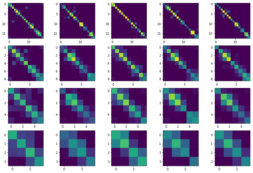
Above, each column is a different spin-z=0 eigenstate, and each row a different blocking. The diagonal of each plot shows the entanglement of each block with its whole environment, and the off-diagonal shows the entanglement with other blocks.