1. schematic - manual drawing

This example demonstrates the basic functionality of the schematic module. The schematic module is a simple wrapper around matplotlib that allows programatically drawing diagrams, e.g. for tensor networks, in 2D and also pseudo-3D. It is used as the backend for automatic drawing in TensorNetwork.draw, but it also useful for making manual diagrams not associated with a tensor network. The main object is the Drawing class.

1.1. Illustrative full examples

The following examples are intended to be illustrative of a full drawing. If you supply a dict of presets to Drawing, then you can provide default styling for various elements simply by name.

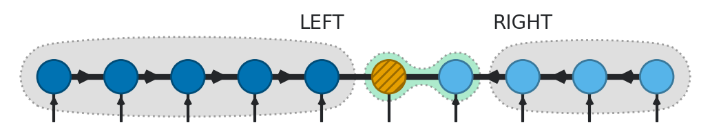
1.1.1. 2D example

%config InlineBackend.figure_formats = ['retina']
from quimb import schematic

presets = {
    "bond": {"linewidth": 3},
    "phys": {"linewidth": 1.5},
    "center": {
        # `get_color` uses more colorblind friendly colors
        "color": schematic.get_color("orange"),
        "hatch": "/////",
    },
    "left": {
        "color": schematic.get_color("bluedark"),
    },
    "right": {
        "color": schematic.get_color("blue"),
    },
}

d = schematic.Drawing(presets=presets)

L = 10
center = 5

for i in range(10):
    # draw tensor
    d.circle(
        (i, 0),
        preset=(
            "center" if i == center else "left" if i < center else "right"
        ),
    )

    # draw physical index
    d.line((i, 0), (i, -2 / 3), preset="phys")

    # draw virtual bond
    if i + 1 < L:
        d.line((i, 0), (i + 1, 0), preset="bond")

    # draw isometric conditions
    if i != center:
        d.arrowhead((i, -2 / 3), (i, 0), preset="phys")
    if i < center - 1:
        d.arrowhead((i, 0), (i + 1, 0), preset="bond")
    if i > center + 1:
        d.arrowhead((i, 0), (i - 1, 0), preset="bond")

# label the left
if center > 0:
    d.text((center - 1, 0.8), "LEFT")
    d.patch_around([(i, 0) for i in range(center)], radius=0.5)

# label pair
if center + 1 < L:
    d.patch_around_circles(
        (center, 0),
        0.3,
        (center + 1, 0),
        0.3,
        facecolor=(0.2, 0.8, 0.5, 0.4),
    )

# label the right
if center + 2 < L:
    d.text((center + 2, 0.8), "RIGHT")
    d.patch_around([(i, 0) for i in range(center + 2, L)], radius=0.5)

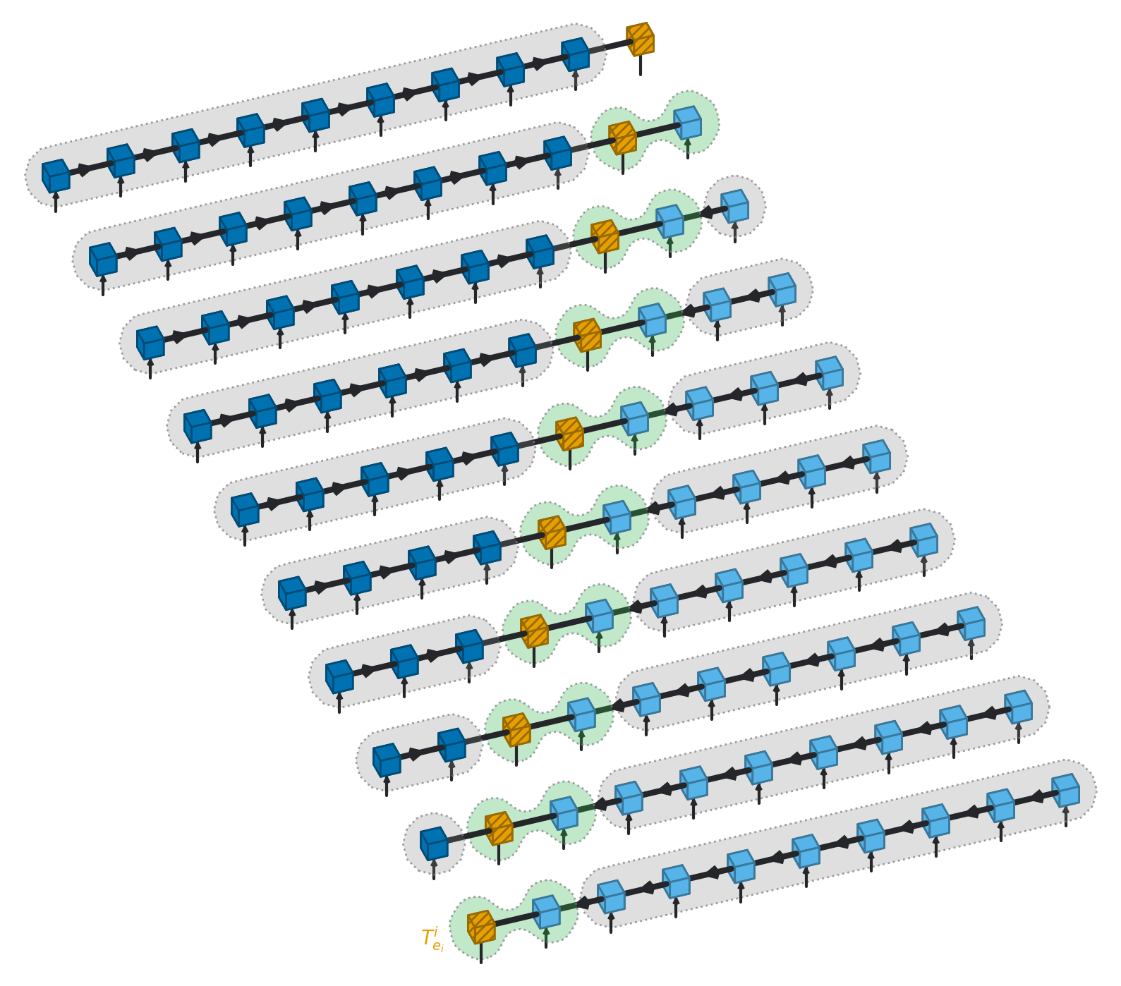
1.1.2. Pseudo-3D example

If you supply 3D coordinates to Drawing methods then the objects will be mapped by the axonometric projection to 2D and given appropriate z-ordering. The projection and orientation can be controlled in the Drawing constructor.

d = schematic.Drawing(presets=presets, figsize=(10, 10))

L = 10

radius = 0.15

for center in range(L):
    # map the stage into a 3D x-coordinate
    x = 2 * center

    for i in range(10):
        # draw tensor, can now use cube rather than circle
        d.cube(
            (i, x, 0),
            radius=radius,
            preset=(
                "center" if i == center else "left" if i < center else "right"
            ),
        )

        # draw physical index
        d.line((i, x, 0), (i, x, -2 / 3), preset="phys")

        # draw virtual bond
        if i + 1 < L:
            d.line((i + radius, x, 0), (i + 1 - radius, x, 0), preset="bond")

        # draw isometric conditions
        if i != center:
            d.arrowhead((i, x, -2 / 3), (i, x, 0), preset="phys")
        if i < center - 1:
            d.arrowhead((i, x, 0), (i + 1, x, 0), preset="bond")
        if i > center + 1:
            d.arrowhead((i, x, 0), (i - 1, x, 0), preset="bond")

    # label the left
    if center > 0:
        d.patch_around(
            [(i, x, 0) for i in range(center)],
            radius=3 * radius,
            smoothing=0.0,
        )

    # label pair
    if center + 1 < L:
        d.patch_around_circles(
            (center, x, 0),
            2.5 * radius,
            (center + 1, x, 0),
            2.5 * radius,
            facecolor=(0.2, 0.7, 0.3, 0.3),
        )

    # label the right
    if center + 2 < L:
        d.patch_around(
            [(i, x, 0) for i in range(center + 2, L)],
            radius=3 * radius,
            smoothing=0.0,
        )

d.text((-3 / 4, 0, 0), "$T^i_{e_i}$", color=schematic.get_color("orange"))

1.2. Individual elements:

Here we demonstrate the different types of individual element that can be placed. The hash_to_color function is useful way to deterministically generate colors from hashable objects.

To help with perspective or placing new items, you can call Drawing.grid() or Drawing.grid3d(), these will use the limits of items placed so far thus should typically be called after.

Hint

Drawing.scale_figsize is another useful method to call last, which scales the absolute figsize of the figure based on the limits of items placed so far. This can be useful for generating sequences of figures where elements are removed and added, but the scale should remain consistent.

import numpy as np

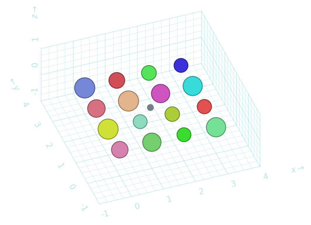
1.2.1. Circles

Drawing.circle draws a circle with a given radius and center coordinates.

d = schematic.Drawing()

coos = [(i, j, 0) for i in range(4) for j in range(4)]

for coo in coos:
    d.circle(
        coo,
        radius=np.random.uniform(0.2, 0.3),
        color=schematic.hash_to_color(str(coo)),
    )

# dot is a simple alias circle
d.dot((1.5, 1.5, 0))

d.grid3d()

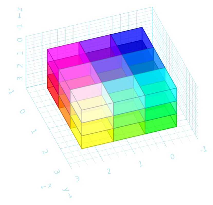
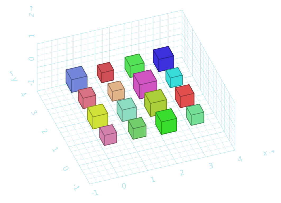
1.2.2. Cubes

Drawing.cube draws a cube with a given ‘radius’ and center coordinates, only for 3D coordinates.

d = schematic.Drawing()

coos = [(i, j, 0) for i in range(4) for j in range(4)]

for coo in coos:
    d.cube(
        coo,
        radius=np.random.uniform(0.2, 0.3),
        color=schematic.hash_to_color(str(coo)),
    )

d.grid3d()

1.2.3. Text

Drawing.text places text in data coordinates (including 3D). Drawing.label_ax and Drawing.label_fig are the same but default to axis and figure coordinates respectively.

d = schematic.Drawing()

coos = [(i, j, 0) for i in range(4) for j in range(4)]

for coo in coos:
    d.text(coo, str(coo), color=schematic.hash_to_color(str(coo)))

# labels are the same but use the axes or figure coordinates
d.label_ax(0.1, 0.9, "$\\mathbf{B}$", fontsize=20)
d.label_fig(0.5, 0.0, "$\\sum_e \\prod_i ~ T^i_{e_i}$", fontsize=16)

d.grid3d()

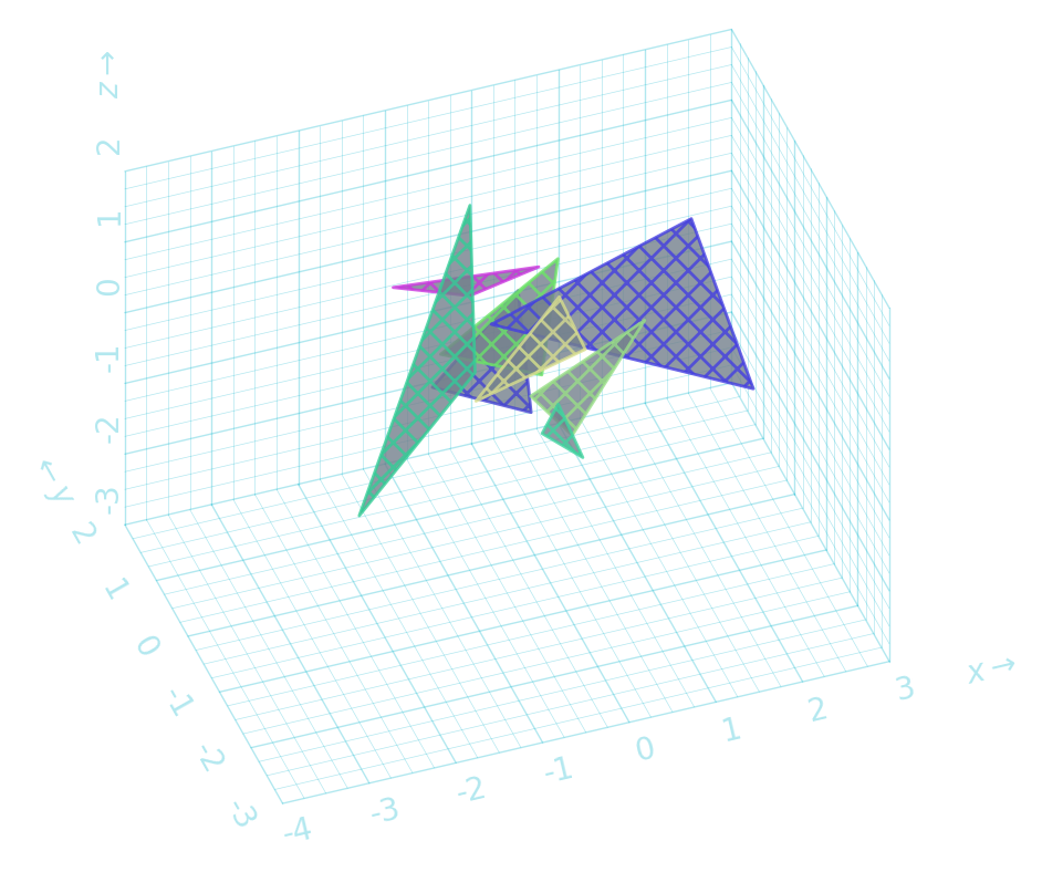
1.2.4. General shapes

Drawing.shape draws a general filled shape given a sequence of 2D or 3D coordinates.

d = schematic.Drawing()

rng = np.random.default_rng(1)
pts = rng.normal(size=(8, 3, 3))

for coos in pts:
    d.shape(
        coos,
        alpha=0.8,
        hatch="XXX",
        edgecolor=schematic.hash_to_color(str(coos)),
    )

d.grid3d()

1.2.5. Markers

Drawing.marker is a convenience method for specifying the shape of a patch using a single string or integer, to yield a regular polygon.

d = schematic.Drawing()

for p in range(3, 10):
    d.marker((p, 0), marker=p)
    d.text((p, 0.5), f"{p}-gon")

d.grid()

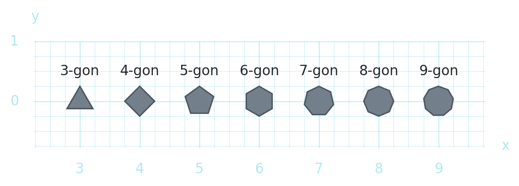
It is a wrapper around Drawing.regular_polygon with which you can also change the rotation with the orientation argument.

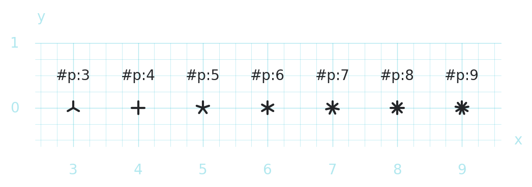
1.2.6. Stars

The other class of markers are drawn using Drawing.star, which you can call directly:

d = schematic.Drawing()

for p in range(3, 10):
    d.star((p, 0), npoint=p)
    d.text((p, 0.5), f"#p:{p}")

d.grid()

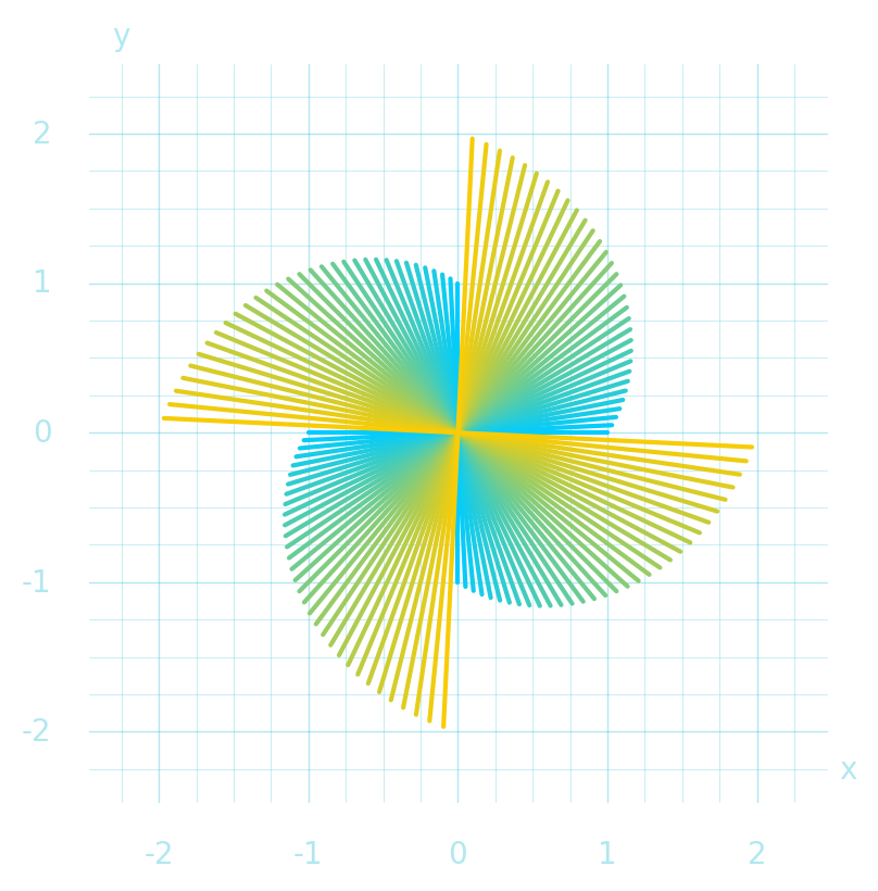
You can specify the radius (in data units) and the orientation (in radians from vertical):

d = schematic.Drawing()

K = 32

for i in range(0, K):
    radius = 1 + i / K
    orientation = i / K * np.pi / 2
    color = (i / K, 0.8, 1 - i / K)
    d.star(
        (0, 0), npoint=4, radius=radius, orientation=orientation, color=color
    )

d.grid()

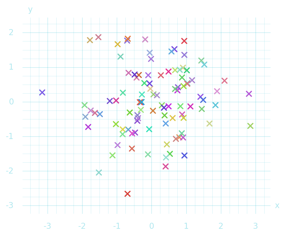
The alias Drawing.cross is shorthand for drawing a diagonal star with 4 points:

d = schematic.Drawing()
coos = np.random.randn(100, 2)
for x, y in coos:
    d.cross((x, y), color=schematic.hash_to_color(str((x, y))))
d.grid()

1.3. Lines and curves

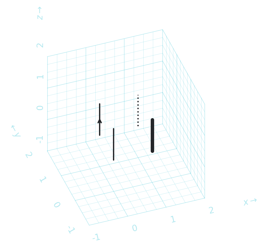
1.3.1. Lines

The basic method for drawing lines between a pair of 2D or 3d points is Drawing.line.

d = schematic.Drawing()

d.line((0, 0, 0), (0, 0, 1))
d.line((0, 1, 0), (0, 1, 1), arrowhead=True)
d.line((1, 0, 0), (1, 0, 1), linewidth=4)
d.line((1, 1, 0), (1, 1, 1), linestyle=":")

d.grid3d()

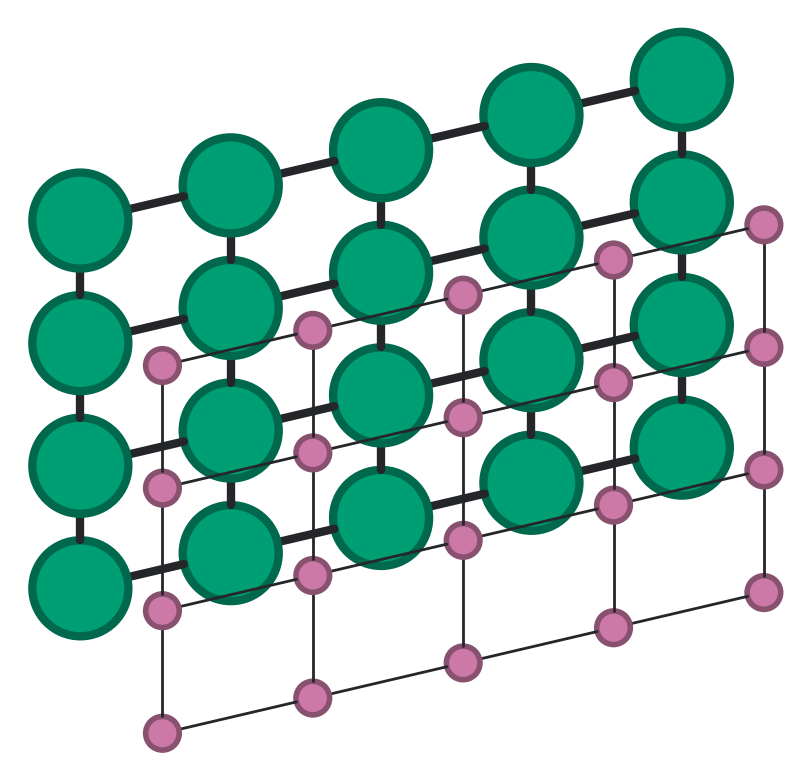
When drawing lattice bonds it can be used fule to shorten the lines somewhat for visual effect.

1. The stretch kwarg applies an overall relative stretch to the whole line.

2. The shorten kwarg makes the line stop an absolute amount shorter, a tuple can be used to control start and end separately.

By setting shorten to the radius of circles drawn, the lines connect exactly to the circle edge:

d = schematic.Drawing()

r = 0.15

edges = [((i, j), (i, j + 1)) for i in range(5) for j in range(3)] + [
    ((i, j), (i + 1, j)) for i in range(4) for j in range(4)
]
sites = {site for edge in edges for site in edge}

for i, j in sites:
    d.circle(
        (i, 0, j),
        radius=2.0 * r,
        color=schematic.get_color("green"),
        linewidth=3,
    )
    d.circle(
        (i, -1.5, j),
        radius=0.7 * r,
        color=schematic.get_color("pink"),
        linewidth=2,
    )
for (ia, ja), (ib, jb) in edges:
    d.line((ia, 0, ja), (ib, 0, jb), shorten=2.0 * r, linewidth=3)
    d.line((ia, -1.5, ja), (ib, -1.5, jb), shorten=0.7 * r, linewidth=1)

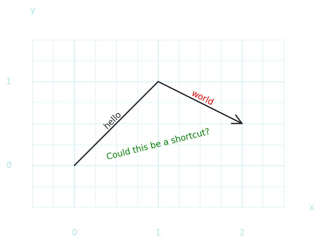
1.3.2. Arrows and labels

You can easily add text and arrows along lines:

d = schematic.Drawing()

pa, pb, pc = (0, 0), (1, 1), (2, 0.5)

d.line(pa, pb, text="hello\n")
d.line(
    pb, pc, text=dict(text="world\n", color="red"), arrowhead=dict(center=1)
)

# calling `line` with `text=` is a shortcut for `text_between`
d.text_between(pa, pc, "Could this be a shortcut?", color="green")
d.grid()

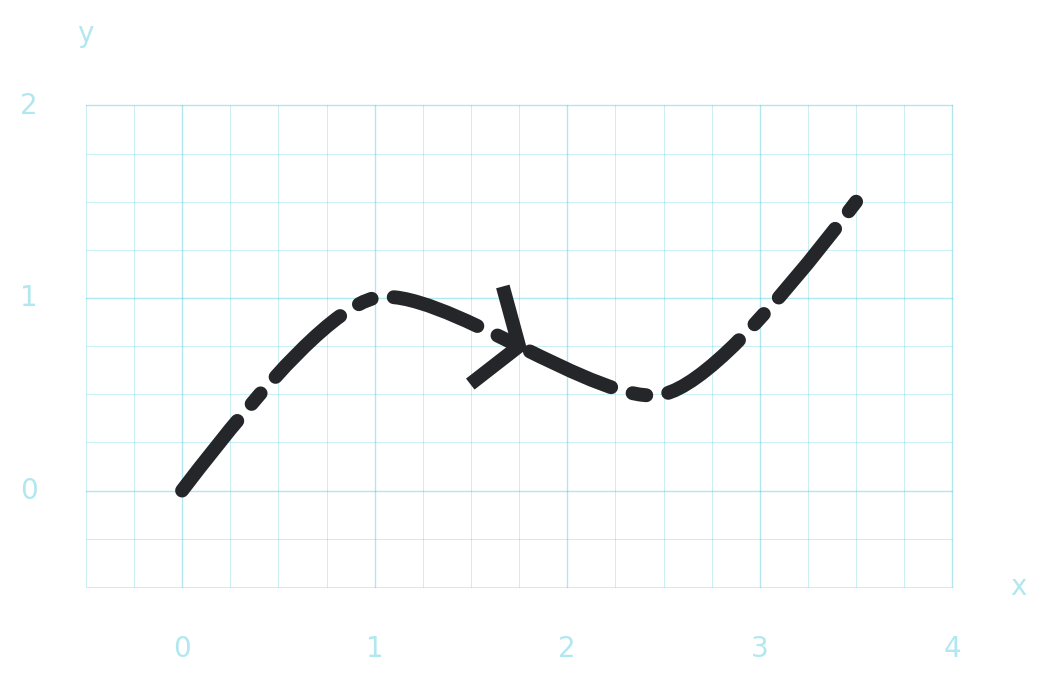
1.3.3. Curves

If you want a line to pass through multiple points, you can use Drawing.curve to draw a smooth curve.

d = schematic.Drawing()

d.curve(
    [(0, 0), (1, 1), (2.5, 0.5), (3.5, 1.5)],
    linestyle="-.",
    linewidth=5,
)

# you can draw just the arrowhead separatel
d.arrowhead((1, 1), (2.5, 0.5), linewidth=5, width=0.15)

d.grid()

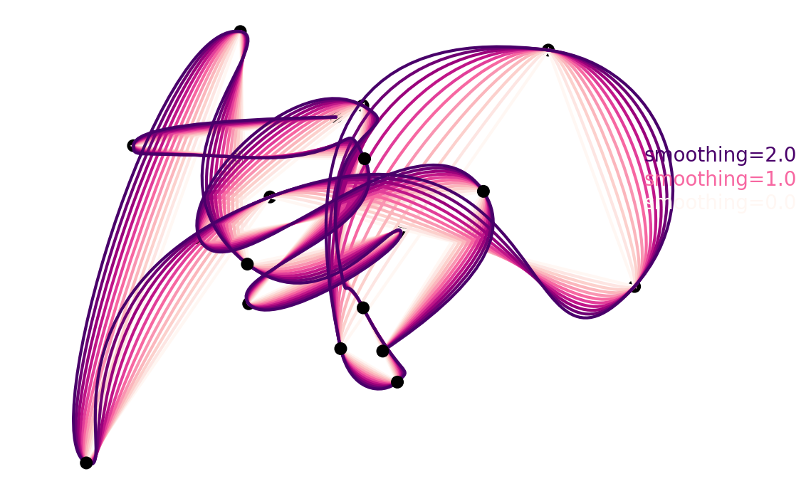
Curves pass exactly through all points given, with the smoothing kwarg controlling… how smoothly they do this.

import matplotlib as mpl

d = schematic.Drawing()

rng = np.random.default_rng(1)
pts = rng.normal(size=(20, 3))
cm = mpl.colormaps.get_cmap("RdPu")

for pt in pts:
    d.dot(pt, color="black", radius=0.05)

for smoothing in np.linspace(0.0, 2.0, 11):
    d.curve(pts, smoothing=smoothing, color=cm(smoothing / 2))

d.label_ax(1.0, 0.60, "smoothing=0.0", color=cm(0.0))
d.label_ax(1.0, 0.65, "smoothing=1.0", color=cm(0.5))
d.label_ax(1.0, 0.70, "smoothing=2.0", color=cm(1.0))

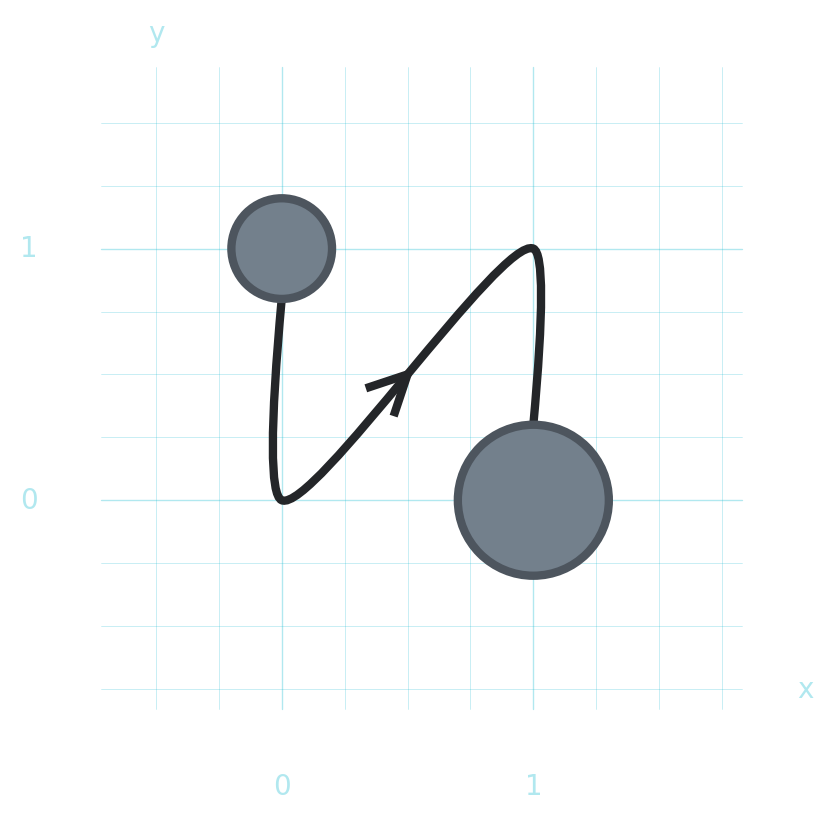
Drawing.curve also takes the shorten kwarg which shortens the final segments by the specified absolute amount:

d = schematic.Drawing()

r1 = 0.2
r2 = 0.3

d.circle((0, 1), radius=r1, linewidth=3)
d.curve([(0, 1), (0, 0), (1, 1), (1, 0)], shorten=(r1, r2), linewidth=3)
# also add an arrow on the middle segment
d.arrowhead((0, 0), (1, 1), linewidth=3)
d.circle((1, 0), radius=r2, linewidth=3)
d.grid()

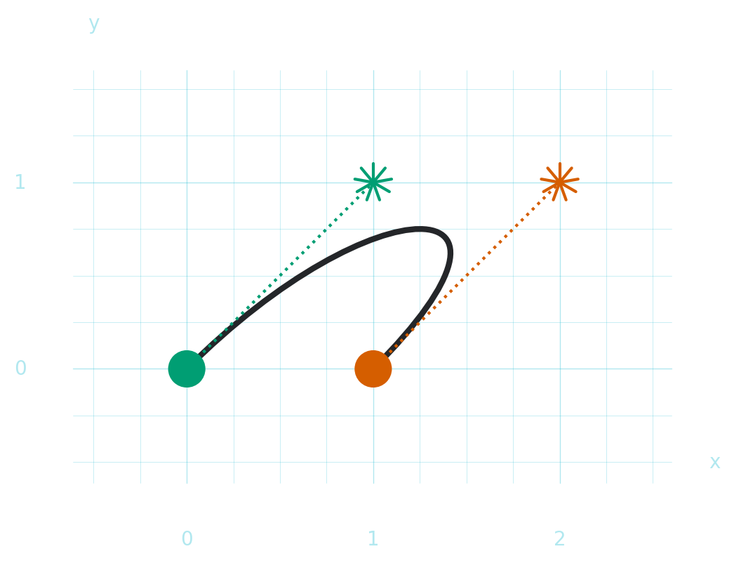
1.3.4. Bezier

If you want to draw a bezier curve by explitly passing both the coordinates and the anchor points you can use Drawing.bezier:

d = schematic.Drawing()

cooa = (0, 0)
anca = (1, 1)
ancb = (2, 1)
coob = (1, 0)

d.bezier([cooa, anca, ancb, coob], linewidth=3)

d.dot(cooa, color=schematic.get_color("green"))
d.star(anca, color=schematic.get_color("green"))
d.line(cooa, anca, linestyle=":", color=schematic.get_color("green"))

d.dot(coob, color=schematic.get_color("red"))
d.star(ancb, color=schematic.get_color("red"))
d.line(coob, ancb, linestyle=":", color=schematic.get_color("red"))
d.grid()

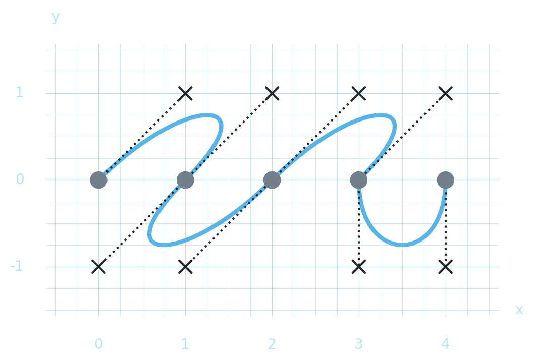
You can supply any sequence of length 3N + 1 to draw a continuous line:

d = schematic.Drawing()

coos = [
    (0, 0),
    (1, 1),
    (2, 1),  # control points
    (1, 0),
    (0, -1),
    (1, -1),  # control points
    (2, 0),
    (3, 1),
    (4, 1),  # control points
    (3, 0),
    (3, -1),
    (4, -1),  # control points
    (4, 0),
]
d.bezier(coos, linewidth=3, color=schematic.get_color("blue"))

for i in range(0, len(coos) - 1, 3):
    d.dot(coos[i])
    d.dot(coos[i + 3])
    d.cross(coos[i + 1])
    d.cross(coos[i + 2])
    d.line(coos[i], coos[i + 1], linestyle=":")
    d.line(coos[i + 2], coos[i + 3], linestyle=":")

d.grid()

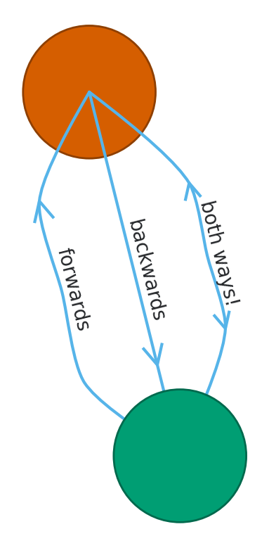
1.3.5. Multi-edges

If you want to programmatically draw multiple lines from one place to the other (‘multi-edges’) you can use Drawing.line_offset:

d = schematic.Drawing()

pa, pb = (0, 0, 0), (0, 1, 1)

green = schematic.get_color("green")
red = schematic.get_color("red")
blue = schematic.get_color("blue")

d.circle(pa, color=green)
d.circle(pb, color=red)

# you can still use arrowheads and text labels
d.line_offset(
    pa, pb, 0.2, arrowhead=dict(center=0.9), text="forwards\n", color=blue
)
d.line_offset(
    pa,
    pb,
    0.0,
    arrowhead=dict(center=0.9, reverse=True),
    text="backwards\n",
    color=blue,
)
d.line_offset(
    pa,
    pb,
    -0.2,
    arrowhead=dict(center=0.9, reverse="both"),
    text="both ways!\n",
    color=blue,
    midlength=0.4,
)

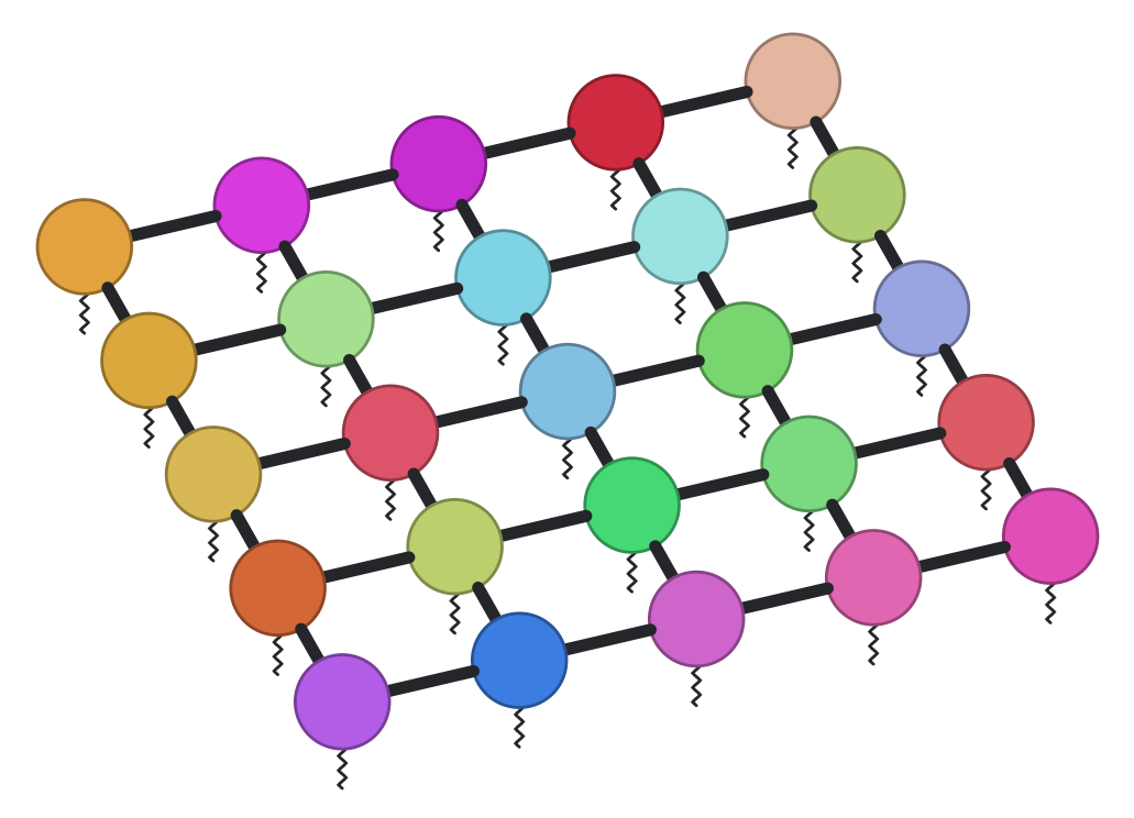
1.3.6. zigzags

Drawing.zigzag is similar to Drawing.line, but creates a zigzag pattern instead of a straight line, which can be useful to differentiate beyond linestyle.

d = schematic.Drawing()

for i in range(5):
    for j in range(5):
        d.circle((i, j, 1), color=schematic.hash_to_color(str((i, j))))
        if i < 4:
            d.line((i, j, 1), (i + 1, j, 1), linewidth=4, shorten=0.25)
        if j < 4:
            d.line((i, j, 1), (i, j + 1, 1), linewidth=4, shorten=0.25)

        d.zigzag((i, j, 1), (i, j, 0.4), linewidth=1, width=0.02)

You can control:

• smoothing: how smooth the zigzagging is (0 = sharp corners, 1 = very smooth)

• extend: only start zigzagging after this length

• width: the width of the zigzag line, by default aims for 8 zigzags

d = schematic.Drawing()
d.zigzag((0, 0), (2, 0), smoothing=0.0, extend=0.3, width=0.03)

1.4. Highlighting areas and groups of objects

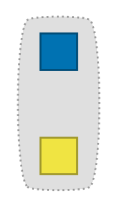
1.4.1. Patches around general areas

In technical drawings it is often useful to highlight areas. The Drawing.patch method does this by filling in a curve, given by a sequence of 2D or 3D coordinates.

d = schematic.Drawing()

d.marker((0, 0), marker="s", color=schematic.get_color("yellow"))
d.marker((0, 1), marker="s", color=schematic.get_color("bluedark"))
d.patch(
    [
        (-0.3, -0.3),
        (+0.3, -0.3),
        (+0.3, +1.3),
        (-0.3, +1.3),
    ],
    smoothing=0.3,
)
d.scale_figsize()

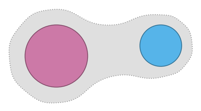
1.4.2. Patches around two circles

If you want to specifically highlight two circles, you can use Drawing.patch_around_circles, and simply specify the two circles by their center coordinates and radii.

d = schematic.Drawing(figsize=(4, 4))

d.circle((0, 0), radius=3, color=schematic.get_color("pink"))
d.circle((10, 1), radius=2, color=schematic.get_color("blue"))

d.patch_around_circles(
    (0, 0),
    3,
    (10, 1),
    2,
    padding=0.5,
)

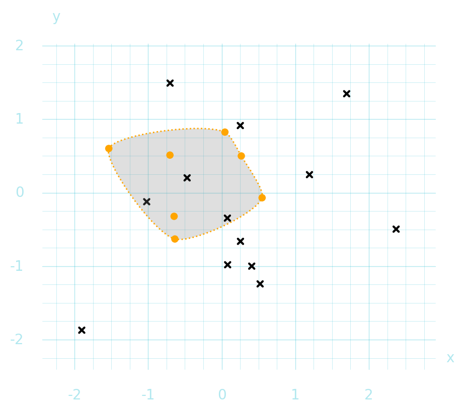
1.4.3. Patches around arbitrary collections of objects

If you want to highlight an arbitrary collection of objects, you can call Drawing.patch_around, this computes the convex hull of the objects and draws a patch around it.

d = schematic.Drawing()

for pt in pts[:7]:
    d.dot(pt, color="orange", radius=0.05)
for pt in pts[7:]:
    d.cross(pt, color="black", radius=0.05)

d.patch_around(pts[:7], edgecolor="orange")
d.grid()

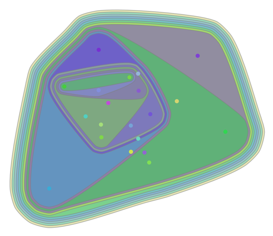
You can control how much padding is added around the perimeter of the objects using the radius kwarg.

d = schematic.Drawing()

for k, pt in enumerate(pts):
    d.dot(pt, color=schematic.hash_to_color(str(k)), radius=0.05)

for k in range(1, len(pts)):
    d.patch_around(
        pts[:k],
        radius=0.05 * k,
        facecolor=schematic.hash_to_color(str(k - 1)),
        linestyle="-",
        zorder=-k,
        alpha=0.5,
    )

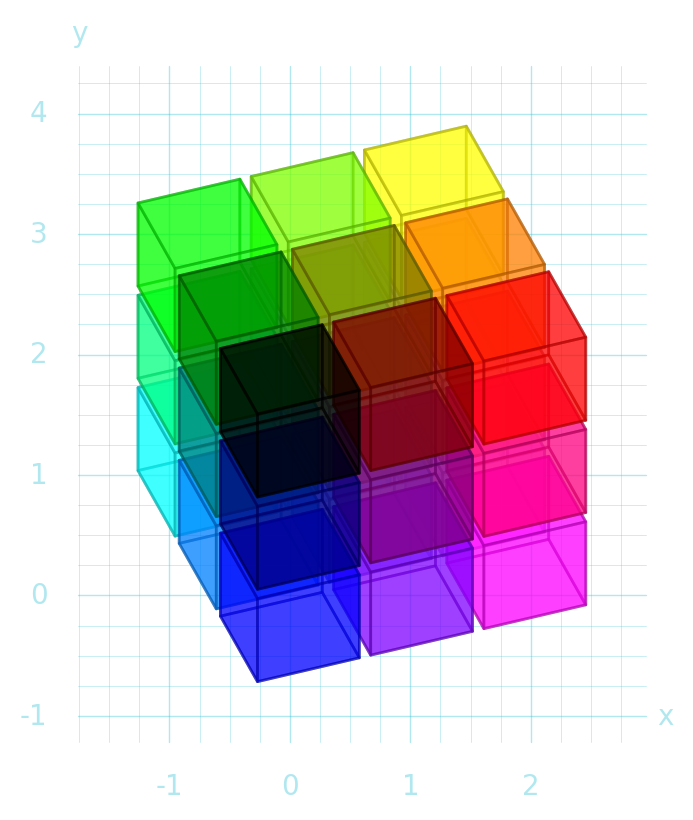
1.5. 3D Projections

schematic can project from 3D coordinates to the 2D plane using either an orthographic (the default) or axonometric projection.

d = schematic.Drawing()
for i in range(3):
    for j in range(3):
        for k in range(3):
            color = (i / 2, j / 2, 1 - k / 2)
            d.cube((i, j, k), color=color, radius=0.45, alpha=0.5)
d.grid()

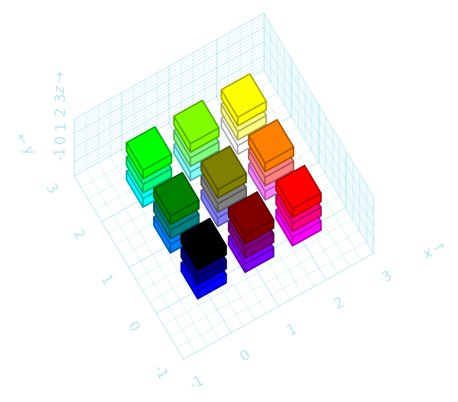
Change the orientation of the ‘camera’:

azimuth = 30  # y-axis 30 degrees to left
elevation = 75  # almost top down
d = schematic.Drawing(projection=(azimuth, elevation))
for i in range(3):
    for j in range(3):
        for k in range(3):
            color = (i / 2, j / 2, 1 - k / 2)
            d.cube((i, j, k), color=color, radius=0.3)
d.grid3d()

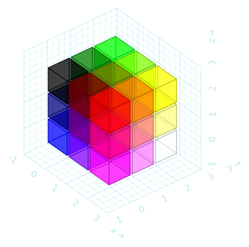
Use axonometric projection and specify angles:

xangle = -35
yangle = +25
d = schematic.Drawing(projection=("axonometric", xangle, yangle))
for i in range(3):
    for j in range(3):
        for k in range(3):
            color = (i / 2, j / 2, 1 - k / 2)
            d.cube((i, j, k), color=color, radius=0.45, alpha=0.5)
d.grid3d()

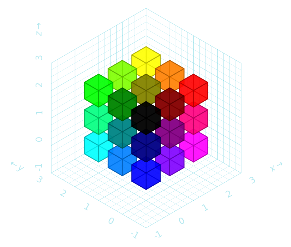
"isometric" is shorthand for angles 30 / 150.

d = schematic.Drawing(projection="isometric")
for i in range(3):
    for j in range(3):
        for k in range(3):
            color = (i / 2, j / 2, 1 - k / 2)
            d.cube((i, j, k), color=color, radius=0.3, alpha=0.7)
d.grid3d()

With both 2D and 3D drawings you can specify xscale, yscale and zscale to apply a simple linear transformation in that direction.

d = schematic.Drawing(
    xscale=-2,  # flip and stretch
    yscale=-2,  # flip and stretch
    zscale=-1,  # flip only
)
for i in range(3):
    for j in range(3):
        for k in range(3):
            color = (i / 2, j / 2, 1 - k / 2)
            d.cube((i, j, k), color=color, radius=0.5, alpha=0.5)
d.grid3d()